 , M. Prange1, 2 and G. Lohmann1, 2
| Climate Dynamics |
| 10.1007/s00382-004-0395-z |
V. Romanova1 , M. Prange1, 2 and G. Lohmann1, 2
| (1) | Geoscience Department, University of Bremen, Klagenfurterstr., 28334 Bremen, Germany |
| (2) | DFG Research Center Ocean Margins (RCOM), University of Bremen, 28334 Bremen, Germany |
|
V. Romanova Email: vanya@palmod.uni-bremen.de |
Received: 10 April 2003 Accepted: 29 December 2003
 s
circulation. The most sensitive part of the hydrological balance
appears to be in the tropical and subtropical regions suggesting that
the
s
circulation. The most sensitive part of the hydrological balance
appears to be in the tropical and subtropical regions suggesting that
the  Achilles heel of the global conveyor belt circulation is not restricted to the northern North Atlantic where convection occurs.
Transporting heat over large distances, the thermohaline circulation (THC) plays a pivotal role in the climate system. Geological records from the Last Glaciation indicate that greater abundances of ice-rafted debris in the North Atlantic (Heinrich Events) were associated with global-scale climatic changes (Broecker and Hemming 2001), probably resulting from a THC slowdown (Boyle and Keigwin 1987; Clark et al. 2002). The concept of THC fluctuations with global impact has motivated a large number of researchers to study the sensitivity of the circulation to North Atlantic meltwater inflow, utilizing numerical climate models (e.g. Bryan 1986; Maier-Reimer and Mikolajewicz 1989; Stocker and Wright 1991; Mikolajewicz and Maier-Reimer 1994; Manabe and Stouffer 1995; Rahmstorf 1995; Lohmann et al. 1996a; Rahmstorf 1996; Fanning and Weaver 1997; Schiller et al. 1997; Rind et al. 2001). In many of these models, the THC possesses multiple equilibria, and transitions from one mode of operation to another can be triggered by a sufficiently strong freshwater perturbation. Consequently, a short-term meltwater influx can have a persistent effect on the THC by inducing a transition from a mode with intense North Atlantic Deep Water (NADW) formation to a mode with weak or ceased convective activity.
In
model experiments, meltwater perturbations were usually applied to
present-day states of the THC. The suitability of such experiments for glacial
conditions has been challenged by results from box models, suggesting
that the weaker overturning circulation of the ice age was more
vulnerable than the modern one (Lohmann et al. 1996b; Prange et al. 1997). A recent study by Ganopolski and Rahmstorf (2001)
provides a new perspective on the stability properties of glacial
climate. Utilizing an earth system model of intermediate complexity,
the authors suggested that the glacial THC possesses only one
equilibrium. This mono-stable behaviour of the THC may explain the
conveyors recovery after a meltwater-induced shutdown associated with a Heinrich Event. The results of Ganopolski and Rahmstorf (2001) were corroborated by Prange et al. (2002),
who demonstrated the mono-stability of the THC in a hybrid-coupled
model with a three-dimensional ocean under glacial conditions. In their
modelling approach, the authors used CLIMAP (1981) surface temperatures with an additional cooling in the tropics to force the atmospheric circulation (Lohmann and Lorenz 2000)
as background climate state. This reconstruction is characterized by an
extensive North Atlantic sea ice cover: the Nordic Seas are ice-covered
the whole year round, and the winter ice cover advances southward to
almost 45°N. More recent reconstructions, however, provide evidence for
a substantially reduced ice coverage with vast ice-free areas in the
Nordic Seas during summer (Weinelt et al. 1996; Paul and Schäfer-Neth 2003).
Extending the work of Prange et al. (2002), this study applies the surface temperature reconstructions of Weinelt et al. (1996) and GLAMAP 2000 (Paul and Schäfer-Neth 2003) in a hybrid-coupled climate model. We shall examine the effects of different glacial sea surface temperature fields on the hydrologic cycle, salinity distributions and the oceanic circulation. In particular, we focus on the stability of the glacial THC and its dependence on the background hydrological cycle.
The work is organized as follows: in Sect. 2, the model and experimental set-up is described. The results are presented in the third section and they are discussed in Sect. 4. Conclusions are drawn in the fifth section.
We use the three-dimensional atmospheric general circulation model (AGCM) ECHAM3/T42 (Roeckner et al. 1992).
It is based on the primitive equations and includes radiation and
hydrological cycle. It has 19 levels and a resolution of 128 × 64
points on a Gaussian grid. The forcing is given by insolation,
following the astronomical theory of Milankovic and CO2
concentration. The orbital parameters for 21,000 years BP are taken to
calculate the insolation pattern, which remains unchanged during the
experiments. The CO2 concentration is fixed to 200 ppm for the glacial simulations and to 345 ppm for the control run (Lohmann and Lorenz 2000). The bottom boundary conditions are given by the Earths orography, including ice sheets (Peltier 1994),
albedo, sea-ice cover and sea surface temperatures. The last two
parameters are taken from three different reconstruction sets. As yet,
the model has no dynamic ice sheets. The model output comprises the
monthly averaged surface freshwater fluxes, surface air temperatures
and wind stresses. The model is run for 15 years of model integration
and averaged years are constructed from the last 10 years of the
simulations.
The
ocean model is based on the LSG ocean circulation model. It integrates
the primitive equations, including all terms except the nonlinear
advection of momentum, using a time step of 1 month (Maier-Reimer et
al. 1993). It has a horizontal resolution of 3.5° × 3.5° and 11 vertical levels on a semi-staggered grid type E.
Parametrization of the density is given by the UNESCO formula. A new
numerical scheme for the advection of temperature and salinity has been
implemented (Schäfer-Neth and Paul 2001; Prange et al. 2003).
It uses a predictor-corrector method, as the predictor step is centred
differences and the corrector step is a third-order QUICK scheme
(Leonard 1979). The advantage of this
scheme is the reduced numerical diffusion in comparison with the
previously used upstream scheme. The vertical diffusivity is prescribed
ranging from 0.6 cm2 s–1 at the surface up to 1.3 cm2 s–1
in the abyssal ocean. The sea level is reduced by 120 m, accounting for
the water stored in the land ice, thus the Bering Strait is closed.
|
 1 and 1 are chosen to be 15 Wm–2 K–1 and 2*1012 W K–1).
In the model, sea surface salinity (SSS) can freely evolve. When the
grid cells are covered by sea ice the surface temperatures are set to
the freezing point.
1 and 1 are chosen to be 15 Wm–2 K–1 and 2*1012 W K–1).
In the model, sea surface salinity (SSS) can freely evolve. When the
grid cells are covered by sea ice the surface temperatures are set to
the freezing point.An extensive parameter study of this hybrid-coupled model approach has been carried out by Prange et al. (2003). It has been shown that this model approach is able to simulate variable sea surface temperatures and salinities and it has been applied to deglaciation scenarios (Knorr and Lohmann 2003; Rühlemann et al. 2004; Prange et al. 2004). The model set-up neglects feedbacks connected with atmospheric dynamics, vegetation and cryosphere.
The
control run is forced with present-day SSTs used in AMIP (Atmospheric
Model Intercomparison Project) and is discussed in Prange et al. (2003). For the glacial we use three different SST and sea-ice reconstruction data sets. Experiment C, the reference experiment, employs CLIMAP (1981) SST and sea ice. This reconstruction uses samples for a time interval between 24 and 14 14C ka BP, in which a climatic stability is assumed (Mix et al. 2001).
An additional tropical cooling of 3 °C is applied in the tropics. It
has been shown that this provides for a consistency with terrestrial
and marine proxy data during the Last Glacial Maximum (LGM) (Farrera et
al. 1999; Lohmann and Lorenz 2000). The second experiment W is forced with SST reconstructions of Weinelt et al. (1996) for the Nordic Seas, combined with the CLIMAP data set (Schäfer-Neth and Paul 2001).
This reconstruction assumes LGM as a period of climatic stability and
minimum meltwater flux for the time interval between 18 and 15 14C ka BP. The data set shows seasonally ice-free conditions in most parts of the Nordic Seas (see Fig. 3b) along with higher summer SST than in the CLIMAP (1981)
reconstruction. A recent reconstruction, GLAMAP 2000 (German Glacial
Atlantic Ocean Mapping Project), comprises the North, Central and South
Atlantic Ocean using joint definitions of the LGM time slice as the
overlap of the Last Isotope Maximum (18-15 14C ka BP) and the EPILOG Level-1 (19-16 14C ka BP) time span, sedimentation rates and resolution (Paul and Schäfer-Neth 2003). A detailed description of the choice of the LGM slice and age control is given in Sarnthein et al. (2003).
It uses 275 sediment cores and the SST estimates are based on a new set
of more than 1000 reference samples of planktonic foraminifera,
radiolarians and diatoms, and on improved transfer-function techniques.
The winter sea ice in the GLAMAP 2000 reconstruction is similar to the
CLIMAP summer sea ice boundary and the Nordic Seas are ice-free during
the summer months (see Fig. 4). The whole year
round, the SSTs are significantly higher in the North Atlantic compared
with the CLIMAP reconstruction. The summer SSTs are considerably higher
around Newfoundland and the Nordic Seas. The simulation using the SSTs
provided by GLAMAP 2000 is indicated by the abbreviation G. The experiments described above are called glacial experiments hereafter.
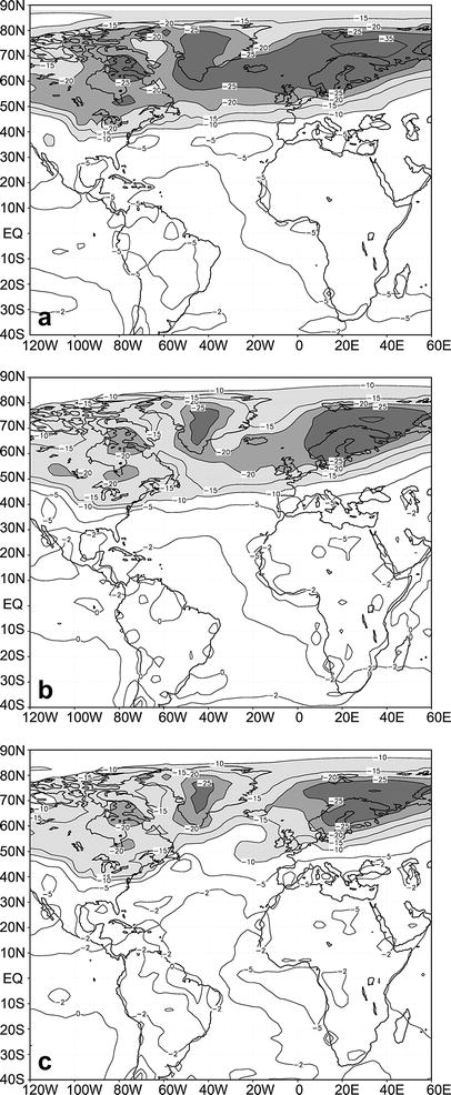
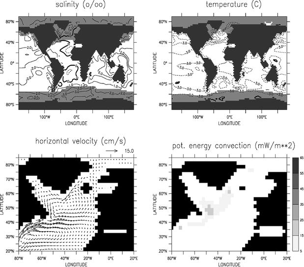
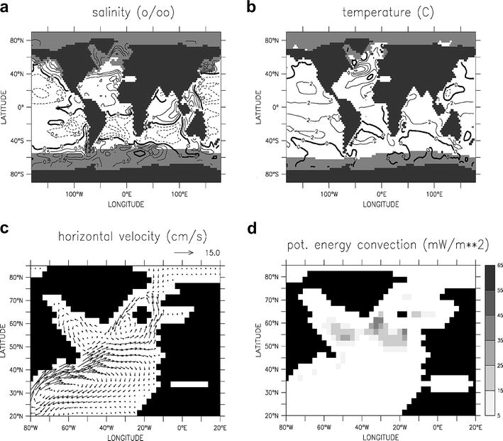
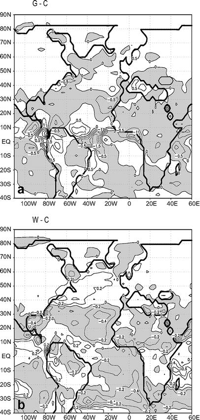
The anomalous salinity field, averaged over the top 150 m for experiment C is shown in Fig. 2a relative to present-day. Taking the global salinity elevation of 1 psu into account, the glacial upper ocean appears relatively fresh. The salinity of the surface waters decreases gradually from the tropics to the north recharging 45°N and further. A salty tongue of 35.0 psu spreads southward of Iceland up to the summer sea ice margin (not shown). The salinity differences of W and G relative to C are shown in Figs. 3a and 4a. A slight salinity increase occurs at 60°N in the southern vicinities of Iceland, favouring NADW formation in these regions. Experiment G shows positive salinity anomalies (around +1 psu) in the Northern Hemisphere and negative anomalies (around –1 psu) in the Southern Hemisphere in the Atlantic relative to experiment C. This enhanced north-south salinity contrast is not representative for experiment W, where the anomalies are positive in the whole Atlantic. In the South Pacific we find a highly saline subtropical gyre (maximum salinity 37.0 psu), and an area of freshwater in the North Pacific (of around 33.0 psu). Therefore, it has formed a bipolar saline-fresh structure opposite to the Atlantic structure, a configuration similar to the present-day distribution. The salinity anomalies W–C and G–C (Figs. 3a and 4a) show fresher conditions in the Pacific. The model simulates an Indonesian salinity maximum in the Indian Ocean and the Western Pacific.
Figure 2b shows annual mean temperature anomalies relative to present-day values, averaged over the uppermost 150 m, for experiment C. Very strong temperature gradients (not shown) are located in the Atlantic between 35°N and 55°N. The temperature front, which is zonal in C (Fig. 2b), is turned to a more meridional direction in experiment W (Fig. 3b) and G (Fig. 4b). Strong anomalies are found near Newfoundland (up to 10 °C) in experiment G.
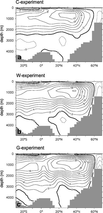
In all three experiments, the subtropical and subpolar Atlantic gyres are well simulated (Figs. 2c, 3c and 4c). The warm North Atlantic Current divides into three parts. The first part flows into the Nordic Seas, circulating around Iceland and, after cooling, the waters head southward through the cold East Greenland Current. This horizontal circulation appears to be stronger for G and W. The second part of North Atlantic waters is advected southwards, to the eastern branch of the subtropical gyre. The third part of the current system circulates cyclonically in the latitudes south of Iceland forming the subpolar gyre. The last type of circulation is particularly strong in C. In conclusion the horizontal circulation for the climates with warm glacial conditions appear more meridionally than in experiment C.
The North Atlantic convection sites (Figs. 2d, 3d and 4d) in the glacial simulations are located near the North American coast, in the Labrador Sea and in the Irminger Sea. The convective areas are between 40°N and 65°N in all cases. This differs from the present-day pattern, simulated with the same model, where the regions of convection are situated mainly in the Nordic Seas and in the Labrador Sea (Prange et al. 2003). The southward displacement of the convection sites in the glacial simulations is associated with a southward shift of NADW formation. In spite of this common general feature, the three experiments differ in convection strength and geographical details in the convective patterns. Convective activity is strongest in experiment G and weakest in experiment C. Investigating the seasonality of the convection, the maximum activity in C is found in autumn, when the temperatures of the surface waters are low enough to form denser waters for convection to start. The required cooling for maximum convection occurs in the early autumn, rather than in winter, due to the low summer temperatures. In experiment G, maximum convection occurs in January, several months later than in C, as a result of the longer time for the necessary surface water cooling. In experiment W, the maximum convection is found in late autumn, as the summer surface waters are warmer than in C, but cooler than in G.
 (Prange et al. 2003; Lohmann 2003). The integral is calculated over the depth,
 is the zonally averaged salinity,
 is the zonally integrated meridional velocity and S0
= 35 psu is a reference salinity. At 30°S, the lowest value of the
freshwater transport due to the overturning is found in experiment C (Fot = 0.034 Sv), followed by experiment W (Fot = 0.054 Sv), and the largest value is found in experiment G (Fot
= 0.072 Sv). When comparing these numbers with the total freshwater
loss, it is concluded that the overturning component of the freshwater
transport is only a minor part of the net evaporation over the
Atlantic.
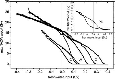
critical point
where the freshwater input causes a complete shutdown of the THC. Then
the freshwater input is decreased so that the circulation recovers.
Afterwards, the freshwater input is increased again in order to return
to the initial state. The resulting hysteresis diagrams for experiments C, W and G are displayed in Fig. 9. In experiment C, an anomalous (critical) freshwater flux of 0.16 Sv is required for a THC shutdown. The critical freshwater input increases for W and G (0.24 Sv and 0.36 Sv, respectively). In Fig. 10 the dependence of the critical
freshwater perturbation on the net evaporation rate is displayed. The
graph suggests a monotonic relationship between the stability of the
ocean circulation and the hydrological budget in the Atlantic Ocean.
is the zonally integrated meridional velocity and S0
= 35 psu is a reference salinity. At 30°S, the lowest value of the
freshwater transport due to the overturning is found in experiment C (Fot = 0.034 Sv), followed by experiment W (Fot = 0.054 Sv), and the largest value is found in experiment G (Fot
= 0.072 Sv). When comparing these numbers with the total freshwater
loss, it is concluded that the overturning component of the freshwater
transport is only a minor part of the net evaporation over the
Atlantic.
critical point
where the freshwater input causes a complete shutdown of the THC. Then
the freshwater input is decreased so that the circulation recovers.
Afterwards, the freshwater input is increased again in order to return
to the initial state. The resulting hysteresis diagrams for experiments C, W and G are displayed in Fig. 9. In experiment C, an anomalous (critical) freshwater flux of 0.16 Sv is required for a THC shutdown. The critical freshwater input increases for W and G (0.24 Sv and 0.36 Sv, respectively). In Fig. 10 the dependence of the critical
freshwater perturbation on the net evaporation rate is displayed. The
graph suggests a monotonic relationship between the stability of the
ocean circulation and the hydrological budget in the Atlantic Ocean.
 critical
 freshwater input for reaching the off-mode
One
could pose the question whether the glacial THC was weaker than the
present-day circulation. In our cold glacial simulation (experiment C)
we find a reduction of 20% of the Atlantic meridional overturning
circulation relative to the present-day simulation (Prange et al. 2003). Utilizing different kinds of coupled models, Weaver et al. (1998), Ganopolski and Rahmstorf (2001), and Shin et al. (2003)
simulated a similar weakening of the conveyor during the glacial
maximum, which is consistent with the geological findings of Rutberg et
al. (2000), who, based on ratios of
neodymium isotopes, reported weakening of NADW export to the Southern
Ocean during the full glacial stages (e.g. LGM), and almost no change
during the warm glacial intervals. A weaker circulation is also
consistent with assimilated paleonutrient tracer distribution in an
ocean circulation model (Winguth et al. 1999). Furthermore, benthic foraminifera  13C,
Cd/Ca and Ba/Ca ratios suggest that the deep Atlantic circulation
during the LGM was influenced by the deep penetration of AABW and
consequent reduction of NADW (Boyle and Keigwin 1987; Duplessy et al. 1988; Boyle 1992; Marchitto et al. 2002).
A shallower overturning cell, approximately 1000 m less than
present-day, is also indicated by the shoaling of the sedimentary
lysocline, which gives the interface between NADW and AABW (Volbers and
Henrich 2003, Frenz and Henrich
submitted 2003). However, the strength of the overturning remains a
controversial topic. No change of the overturning rate is inferred from
sedimentary records of 231Pa/230Th (Yu et al. 1996)
and a new reconstruction combining 55 benthic foraminiferal stable
carbon isotopes suggests no considerable difference to the present-day
circulation strength (Bickert and Mackensen 2003).
On the other hand, three-dimensional coupled models even resulted in
intensification of the LGM ocean circulation (Hewitt et al. 2001; Kitoh and Murakami 2001). Our simulations with warm glacial background conditions (W and G) also exhibit stronger (around 50%) overturning compared to the present-day simulation in Prange et al. (2003).
13C,
Cd/Ca and Ba/Ca ratios suggest that the deep Atlantic circulation
during the LGM was influenced by the deep penetration of AABW and
consequent reduction of NADW (Boyle and Keigwin 1987; Duplessy et al. 1988; Boyle 1992; Marchitto et al. 2002).
A shallower overturning cell, approximately 1000 m less than
present-day, is also indicated by the shoaling of the sedimentary
lysocline, which gives the interface between NADW and AABW (Volbers and
Henrich 2003, Frenz and Henrich
submitted 2003). However, the strength of the overturning remains a
controversial topic. No change of the overturning rate is inferred from
sedimentary records of 231Pa/230Th (Yu et al. 1996)
and a new reconstruction combining 55 benthic foraminiferal stable
carbon isotopes suggests no considerable difference to the present-day
circulation strength (Bickert and Mackensen 2003).
On the other hand, three-dimensional coupled models even resulted in
intensification of the LGM ocean circulation (Hewitt et al. 2001; Kitoh and Murakami 2001). Our simulations with warm glacial background conditions (W and G) also exhibit stronger (around 50%) overturning compared to the present-day simulation in Prange et al. (2003).
Using different SST reconstructions, we are able to detect different glacial salinity distributions at the surface and in the depth. In experiment C, the SSS field shows a tongue of salty waters deeply penetrating from the subtropics to the southern vicinities of Iceland, a feature consistent with the reconstructions of Duplessy et al. (1991). For warm background conditions (W and G) a salinity increase in the Irminger Sea is responsible for the stronger convection and NADW formation. The modelled salinities in the North Atlantic are more consistent with the reconstructions of Duplessy et al. (1991) for both types of experiments with warm (W and G) and cold (C) conditions, and they differ substantially (by more than 1.5 psu) from the values suggested by de Vernal et al. (2000). The mean surface salinity of the glacial ocean appears relatively fresh compared to the present one in our model. The salinity excess of the glacial ocean (+1 psu) is mainly stored in the abyssal ocean, consistent with geological evidence (Adkins et al. 2002).
All experiments for the glacial ocean yield an Atlantic Ocean saltier than the Pacific, similar to the present-day configuration. However, the model study of Lautenschlager et al. (1992) finds the opposite contrast with the Pacific Ocean being saltier than the Atlantic. The simulations of the present-day climate with reduced greenhouse gases, performed by Shin et al. (2003), show also the opposite contrast, but their coupled LGM simulation reveals a fresher Pacific and a saltier Atlantic Ocean relative to present day. An intensification of the salinity contrast between the Atlantic and Pacific oceans is found in experiments G and W relative to C, which originates from strongly increased moisture export out of the Atlantic to the Pacific Ocean. In experiment C, Lohmann and Lorenz (2000) attributed this to enhanced water vapour transport over Panama, reduced water input over the dry African continent and a smaller water vapour import over the North American continent. The latter effect is linked to the presence of the large continental ice-sheets.
Perturbations
of the glacial THC with different climatic background states result in
different hysteresis maps. At zero freshwater input, the glacial THC
has one stable equilibrium only. This can be directly inferred from the
hysteresis curves for experiments W and G (Fig. 9). The weak bistability at zero freshwater input in experiment C is caused by the relative high freshwater flux perturbation rate of 10–4 Sv/year compared to our previous work where we found a strict monostability at the zero point (Prange et al. 2002).
In each experiment, the freshwater budget reveals a net evaporation
over the Atlantic (including Arctic) catchment area with different
strengths. The experiments show that higher net evaporation tends to
shift the equilibrium to a more stable state. The hystereses show that
the coldest climate is more sensitive to freshwater changes than the
warm glacial climates. The salinity enhancement along the conveyor
route through the subtropics induces a northward freshwater transport
across 30°S compensating the freshwater loss from the evaporation. It
may be split into an overturning component, a component related to the
gyre circulation, and a term related to diffusion. The small values,
which are found for the overturning component, suggest that gyre and
diffusive transports play an important role for the stability of the
THC. Consistent with Saenko et al. (2002), Fot
is a poor measure for the stability of the conveyor. During glacial
times, the salinity and temperature induced density gradients between
the North and South Atlantic act in one direction driving the conveyor,
which corresponds to the thermo-haline regime of the ocean system
according to Rahmstorfs (1996) definition. The strong salinity contrast between the South Atlantic and the North Atlantic in experiment G is associated with a stronger haline-driven ocean circulation. The haline factor is weaker in experiment W,
which is partly compensated by the thermal forcing. The predomination
of the haline mechanism induces a stabilizing effect on the THC, which
allows only one stable state of the circulation, namely an on-mode with
NADW formation.
We relate the critical
freshwater input, which causes the collapse of the circulation, to the
hydrological background conditions. The lower evaporation rates over
the Atlantic basin in the cold glacial climate of experiment C
results in a less stable circulation, while the warmer climates with
higher Atlantic net evaporation are more stable. In this sense, the
stability parameters depend explicitly on the background hydrology with
a monotonic (almost linear) relation between the Atlantic evaporation
rates and the critical perturbation.
The glacial THCs substantially differ from the present-day circulation. Using present-day forcing, our model produces a THC with two stable equilibria (Prange et al. 2003), like many other models. Freshwater perturbations can shut down the overturning irrevocably. In the present-day ocean, the THC is driven by SST gradients, while salinity gradients across the Atlantic Ocean tend to weaken the overturning, which allows multiple equilibria of the ocean circulation in the thermal flow regime (Stommel 1961; Rahmstorf 1996). In a coupled three-dimensional OGCM with an energy-moisture balance model for the atmosphere including an ice sheet component, the glacial THC possesses different stability properties (Schmittner et al. 2002). As the ice sheet component in this model set-up does not permit the system to settle into equilibrium, this glacial ocean is characterized by a mode different than the one studied here. In the absence of anomalous freshwater fluxes, their experiments showed only one stable glacial mode, namely the off-mode.
In this study we performed three glacial simulations using three different reconstructions of SST and sea-ice margin as forcing fields for an AGCM. One reconstruction, based on CLIMAP (1981) with additional tropical cooling generates a cold glacial climate equilibrium, whereas the Weinelt et al. (1996) and GLAMAP 2000 (Paul and Schäfer-Neth 2003) reconstructions produce relatively warm glacial climate backgrounds in the North Atlantic realm. In contrast to the present-day THC, all equilibrium states of the simulated LGM climates show a mono-stable behaviour, which can serve as an explanation for the recovery of the THC after meltwater-induced shutdowns (Ganopolski and Rahmstorf 2001; Prange et al. 2002).
In
the differing glacial climate backgrounds, the warm climates show
higher stability than the cold climate. By analyzing the hydrological
balance in the Atlantic catchment area, we find a monotonic dependence
between the Atlantic net evaporation and the critical
freshwater input in the hysteresis causing a complete collapse of the
THC. We conclude that the background hydrological balance plays a
crucial role for the stability of the ocean circulation and, hence, of
the glacial climate. Since THC changes sensitively depend on the
climatic background state with its associated hydrological cycle, our
modelling strategy, employing an AGCM in T42 resolution with explicitly
resolved hydrological cycle seems to be appropriate. This suggests an
important role of the low-latitude hydrological cycle for the branching
and sensitivity of the THC. Such a hydrological bridge and its changes
have been attributed to changes of interannual variability in the
tropical Pacific Ocean (Latif et al. 2000; Schmittner and Clement 2002) as well as to times of weak overturning causing enhanced water vapour transport over the Isthmus of Panama (Lohmann 2003).
Moreover, changes in the South Atlantic, connected with the cold and
warm water routes of the global ocean circulation (Gordon 1986) may strongly determine the regime of the THC (Knorr and Lohmann 2003).
In our model set-up, we have neglected feedbacks connected with atmosphere dynamics, vegetation and the cryosphere. Changes in the hydrological balance are estimated to be in the order of 0.15 Sv, when comparing the climate state of the on and off mode in a coupled atmosphere–ocean general circulation model (Lohmann 2003). The cryosphere provides a great uncertainty. Iceberg discharge has been estimated to be of order 0.15 Sv for 500–1000 years (Calov et al. 2002; Chappell 2002). The effect of vegetation cover on the interocean basin water vapour transport has not been analyzed so far.
In this study, we have not addressed the extent to which the climatic templates represent real glacial climate states. One could speculate that the modelled THC states may possess features of stadial and interstadial circulations, respectively. The different hydrological budgets during relatively cold and warm background conditions would then imply different sensitivities with respect to Heinrich Events (cold conditions) and the Younger Dryas (about 13,000-11,500 years BP), a cold phase which directly followed the warm Bølling-Allerød period. Our study emphasizes the importance of the tropical hydrological cycle, which may provide a possible link between the low latitudes and the ocean circulation on paleoclimatic time scales. In order to understand these linkages, more geological data for the tropical regions is required.

 18O of the glacial deep ocean. Science 298: 1769–1773