Climate Change II
Lecture: April 14, 2026, 9:00 Prof. Dr. Gerrit Lohmann
Preparation
trailer Cellules de Bénard (1min)
Rayleigh–Bénard convection: cooking oil and small aluminium particles (5 min)
Simulations:
Rayleigh Benard Thermal Convection with LBM (5 min)
Rayleigh Benard
Thermal Convection 3D Simulation (2 min)
Exercise advection
The temperature at a point 50 km north of a station is 3\(^\circ\)C cooler than at the station. If the wind is blowing from the northeast at 20m/s and the air is being heated by radiation at a rate of 1\(^\circ\)C/h, what is the local temperature change at the station?
Solution of Temperature Advection
The total change of temperature is given by \[ \frac{d T}{dt} = \frac{\partial T}{\partial t} + {\bf u} \cdot \nabla T = \dot{q} \] \[ \Leftrightarrow \quad \frac{\partial T}{\partial t} = - {\bf u} \cdot \nabla T + \dot{q} \] Here we use the velocity \[ {\bf u} = - 20 \frac{m}{s} \cdot \frac{1}{\sqrt{2}} \quad \left(\begin{array}{c} 1 \\ 1 \\ 0 \end{array}\right) \] \[ \nabla T = \frac{{3}{^\circ C}}{{50}{km}} \left(\begin{array}{c} 0 \\ -1 \\ 0 \end{array}\right) \] \[ \dot{q} = 1 \frac{^\circ C}{h} \] Then we calculate the temperature change at the station \[ \frac{\partial T}{\partial t} = - {\bf u} \cdot \nabla T + \dot{q} \]
\[ \frac{\partial T}{\partial t} = 20 \frac{m}{s} \, \frac{1}{\sqrt{2}} \left(\begin{array}{c} 1 \\ 1 \\ 0 \end{array}\right) \cdot \left(\begin{array}{c} 0 \\ -1 \\ 0 \end{array}\right) \frac{{3}{^\circ C}}{{50}{km}} + 1 \frac{^\circ C}{h} \approx {-2.1} \frac{^\circ C}{h} \]
Rayleigh-Benard convection (and Rayleigh number)
Experiments:
Rayleigh–Bénard convection: cooking oil and small aluminium particles (5 min),
Rayleigh Benard
Thermal Convection 3D Simulation (2 min)


Bifurcations
Bifurcation
youtube, Bifurcation Khan
academy, Bifurcation
K
Max and
Moritz, not lazy, sawing secretly a gap in the bridge.
When now
this act is over, you suddenly hear a scream:
“Hey, out! You billy
goat!
Tailor, tailor, bitch, bitch, bitch!”

Bridge of Schneider Böck: Stability - Instability
And there he is on the bridge,
Cracks! The bridge is falling
apart;

Linear stability analysis
Consider the continuous dynamical system described by \[ \dot x=f(x,\lambda)\quad \] A bifurcation occurs at \[(x_E,\lambda_0)\] if the Jacobian matrix \[ \textrm{d}f/dx (x_E,\lambda_0)\] has an Eigenvalue with zero real part.
Example: transcritical bifurcation
a fixed point interchanges its stability with another fixed point as the control parameter is varied. Bifurcation at \(r=0\).
\[ \frac{dx}{dt}=rx (1-x) \, \]
The two fixed points are 0 and 1. When r is negative, the fixed point at 0 is stable and 1 is unstable. But for \(r>0\), 0 is unstable and 1 is stable.
Stability - Instability: Consumer-producer problem
A typical example could be the consumer-producer problem where the consumption is proportional to the (quantity of) resource.
For example:
\[ \frac{dx}{dt}=rx(1-x)-px \]
where
\[ rx(1-x) \]
is the logistic equation of resource growth:
Rate of reproduction proportional to the population, available resources
\(px\): Consumption, proportional to the resource x.
\[ x_{E 1} = 0, \mbox{ and } x_{E 2 } = 1 - \frac{p}{r} \]
Logistic equation of population growth
Verhulst: describe the self-limiting growth of a biological population with size N:
\[ \frac{dN}{dt}=r N \cdot \left( 1- \frac{N}{K} \right) \]
r growth rate and K carrying capacity.
the early, unimpeded growth rate is modeled by the first term \(r N.\)
“Bottleneck” is modeled by the value of K.
As the population grows, \(-r N^2/K\) becomes large as some members interfere with each other by competing for some critical resource (food, living space). The competition diminishes the combined growth rate, until the value of N ceases to grow (maturity of the population).
\[ N(t) = \frac{K N_0 e^{rt}}{K + N_0 \left( e^{rt} - 1\right)} = \frac{K }{K/N_0 e^{-rt} + 1- e^{-rt} } \quad \rightarrow_{t\to \infty } K \]
In climate, the logistic equation is also important for Lorenz’s forecast error.
Climate Model: Ice-albedo
We use the equilibrium condition:
\[ S(T) = \frac{A + BT}{1 - \alpha(T)} \]
with a smooth albedo function:
\[ \alpha(T) = \alpha_{\text{ice}} - \frac{\alpha_{\text{ice}} - \alpha_{\text{water}}}{2} \left(1 + \tanh\left(\frac{T - T_c}{\Delta}\right)\right) \]
Saddle-node bifurcation: two fixed points collide
3) Potential or Lyapunov Method
\[ \frac{dx}{dt}=b+x^2 = - \frac{d}{dx} \left( - b x - \frac{x^3}{3} \right) = - \frac{d}{dx} V (x) \]

Global analysis including basins of attraction for \(x_{E2}: (-\infty,3)\)
dev.new(width=5, height=4, unit=“cm”) \[ x_{E1} = 2\sqrt{9} = 6 \quad \mbox{unstable} \]
\[ x_{E1} = -2\sqrt{9} = -6 \quad \mbox{stable} \]
4) Graphical method: slope at equilibrium points
\[ \frac{dx}{dt}=b+x^2 \]

filled points: positive slope => unstable
open points: negative slope => stable
Convection in the Rayleigh-Benard system

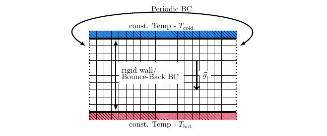
Rayleigh (1916) temperature difference between the upper- and lower-surfaces \[ T(x, y, z=H) = \, T_0 \] \[ T(x, y, z=0) \, = \, T_0 + \Delta T \]
common feature of geophysical flows
No Convection Equilibrium: Diffusion
Diffusion: Temperature varies linearly with depth:
\[ T_{eq} = T_0 + \left(1 - \frac{z}{H}\right) \Delta T \]
No movement of particles:
\[ u = w= 0 \]
When this solution becomes unstable, convection should develop.
No Convection Equilibrium: Diffusion
Rayleigh-Bénard convection and bifurcation
Experiments:
trailer
Cellules de Bénard (1min),
Rayleigh–Bénard
convection made with mix of cooking oil and small aluminium
particles (5 min),
Was haben
Benard-Zellen mit Kochen zu tun? (3 min, German)
Simulations:
Rayleigh Benard
Thermal Convection with LBM (5 min),
Rayleigh Benard
Thermal Convection 3D Simulation (2 min)
Sketch,
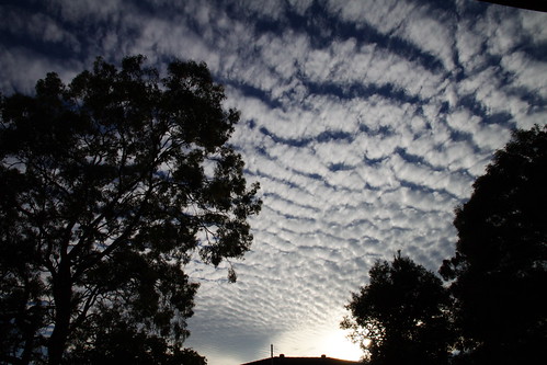
Clouds,
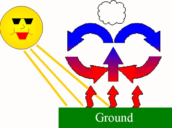
Cartoon
Bifurcations
Bifurcation
youtube (20 min)
Bifurcation Khan
academy (13 min) Reading
Bifurcation theory
Temperature in the Rayleigh-Benard system
\[ T_{eq} = T_0 + \left(1 - \frac{z}{H}\right) \Delta T \]
as an outlook: Conveyor Belt

outlook: Thermohaline ocean circulation

Modelled meridional overturning streamfunction in Sv 10^6 = m^3 /s in the Atlantic Ocean. Grey areas represent zonally integrated smoothed bathymetry
Estimates of overturning ?
It is observed that water sinks in to the deep ocean in polar regions of the Atlantic basin at a rate of 15 Sv. (Atlantic basin: 80,000,000 km^2 area * 4 km depth.)
– How long would it take to ‘fill up’ the Atlantic basin?
– Supposing that the local sinking is balanced by large-scale upwelling, estimate the strength of this upwelling.
Hint: Upwelling = area * w
– Compare this number with that of the Ekman pumping!
Estimates of overturning: Solution
Timescale T to ‘fill up’ the Atlantic basin:
\[ T = \frac{ 80 \cdot 10^{12} \, m^2 \cdot 4000 \, m}{15 \cdot 10^6 \, m^3 s^{-1}} = 2.13 \cdot 10^{10} s = 676 \;years\]
Overturning is balanced by large-scale upwelling:
\[ area \cdot w = 15 \cdot 10^6 \, m^3 s^{-1}\]
\[ w = 0.1875 \cdot 10^{-6} m\;s^{-1} = 5.9 \cdot 10^{-15} m \; y^{-1}. \]