Dynamics II: lecture 3
Gerrit Lohmann date: April 26, 2021
Organization of
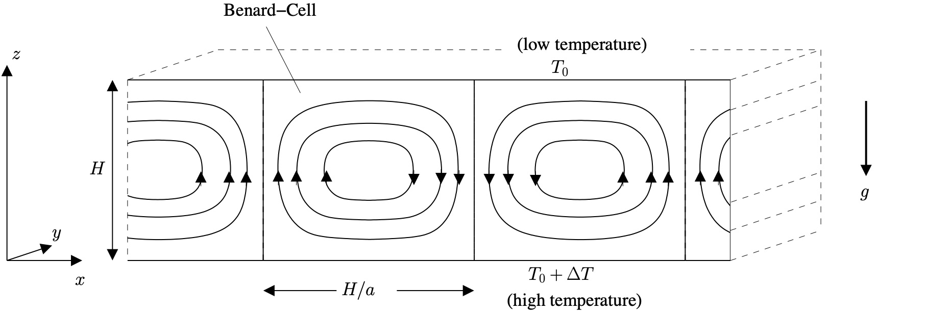
Rayleigh number Ra: Buoyancy & Viscosity
\[ \mbox{Motion develops if } \quad R_a = \frac{g \alpha H^3 \Delta T}{\nu \kappa} \quad \mbox{exceeds } \quad R_c = \pi^4 \frac{(1+a^2)^3}{a^2} \]
\[ \mbox{The minimum value of $R_c = 657.51$ occurs when $a^2 = 1/2$. } \]
\[ \mbox{When } R_a < R_c,\mbox{ heat transfer is due to conduction} \]
\[ \mbox{When } R_a > R_c, \mbox{ heat transfer is due to convection.} \]
Lorenz system
Lorenz system r=24


Scaling: Rotating frame of reference
Scaling: Rotating frame of reference
Rossby number Ro
The local coordinate system
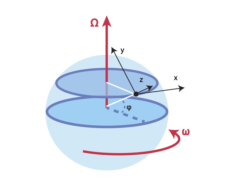
x: east, y: north, z: vertically upwards. \[ (x,y,z)= (a \lambda \cos \varphi, a \varphi, z) \] \( (\lambda,\varphi,z) \) longitude, latitude, height. \( \mbox{Earth radius } a, \Omega \mbox{ rotation } 2 \pi/(24 h) \)
The local coordinate system
x: east, y: north, z: vertically upwards. \[ (x,y,z)= (a \lambda \cos \varphi, a \varphi, z) \] \( (\lambda,\varphi,z) \) longitude, latitude, height.
\( \mbox{Earth radius } a, \Omega \mbox{ rotation } 2 \pi/(24 h) \)
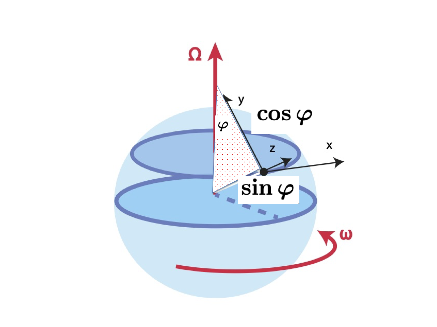
Centrifugal term & Gravitational potential
x: east, y: north, z: vertically upwards. \[ (x,y,z)= (a \lambda \cos \varphi, a \varphi, z) \] \( (\lambda,\varphi,z) \) longitude, latitude, height.
\( \mbox{Earth radius } a, \Omega \mbox{ rotation } 2 \pi/(24 h) \)
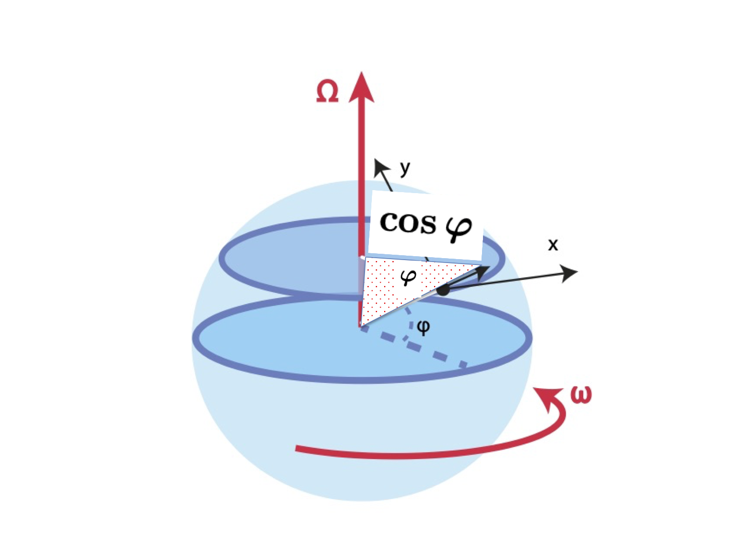
Coriolis acceleration
\[ \boldsymbol{ a}_C =-2\boldsymbol{\Omega \times v}= 2\,\Omega\, \begin{pmatrix} v \sin \varphi- w \cos \varphi \\ -u \sin \varphi \\ u \cos\varphi\end{pmatrix}\ \approx 2\,\Omega\, \begin{pmatrix} v \sin \varphi \\ -u \sin \varphi \\ u \cos\varphi\end{pmatrix}\ \]
For v = 0 and positive \( \varphi \): movement to the east results in acceleration to south.
For u = 0, a movement due north results in an acceleration due east.
Acceleration always is turned \( 90^\circ \) to the right on the Northern Hemisphere

Momentum equations
Momentum equations
Geostrophy
Geostrophy
Large-scale motion:
Perpendicular to the pressure gradient
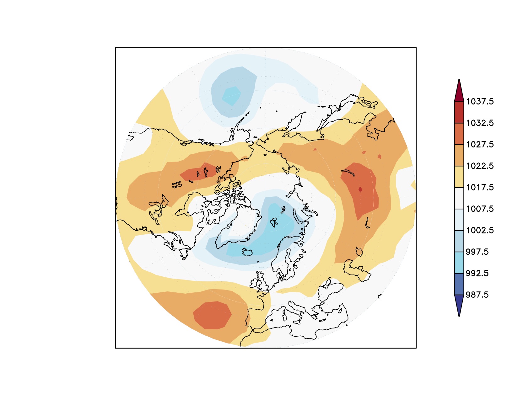
Sea level pressure (hPa) February 2015
Vorticity is the rotation of the fluid
Vorticity is the rotation of the fluid
Example: Vorticity for a rigid body
Example: Vorticity for a rigid body in x direction
Example: Vorticity for a rigid body in y direction
Example: Vorticity for a rigid body in z direction
Example: Vorticity for a rigid body
Example: Vorticity for a rigid body
Example: Vorticity from shear
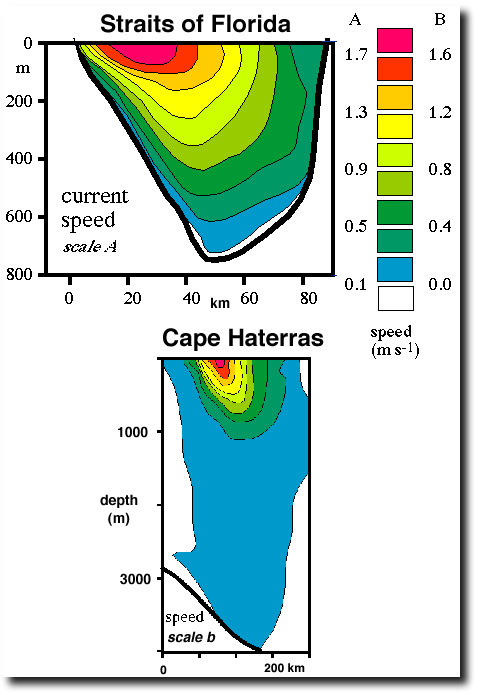
Tomczak & Godfrey: Regional Oceanography
Planetary and relative vorticity
Planetary and relative vorticity
Examples for Vorticity: Ocean with depth h(x,y)
Conservation of Vorticity
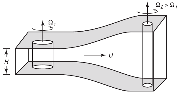
Sketch of the production of relative vorticity by change in the height of a fluid column. As the vertical fluid column moves from left to right, vertical stretching reduces the moment of inertia of the column, causing it to spin faster.
Source: Steward, Oceanography
Conservation of Vorticity
Sketch of the production of relative vorticity by change in the height of a fluid column. As the vertical fluid column moves from left to right, vertical stretching reduces the moment of inertia of the column, causing it to spin faster.
Source: Steward, Oceanography
Conservation of Vorticity
Sketch of the production of relative vorticity by change in the height of a fluid column. As the vertical fluid column moves from left to right, vertical stretching reduces the moment of inertia of the column, causing it to spin faster.
Source: Steward, Oceanography
Conservation of Vorticity
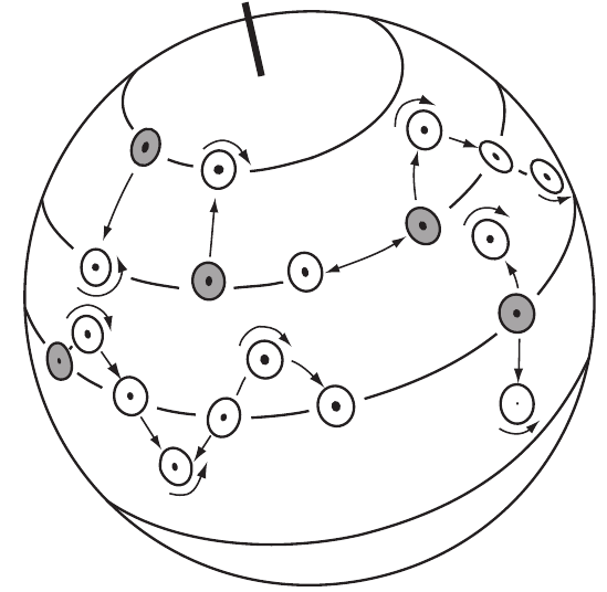
Vorticity tends to be conserved as columns of water change latitude. After von Arx (1962).
\[ \frac{D}{Dt}\left( \zeta+f\right) = 0 \]
Conservation of Vorticity
Vorticity tends to be conserved as columns of water change latitude. After von Arx (1962).
\[ \frac{D}{Dt}\left( \zeta+f\right) = 0 \]
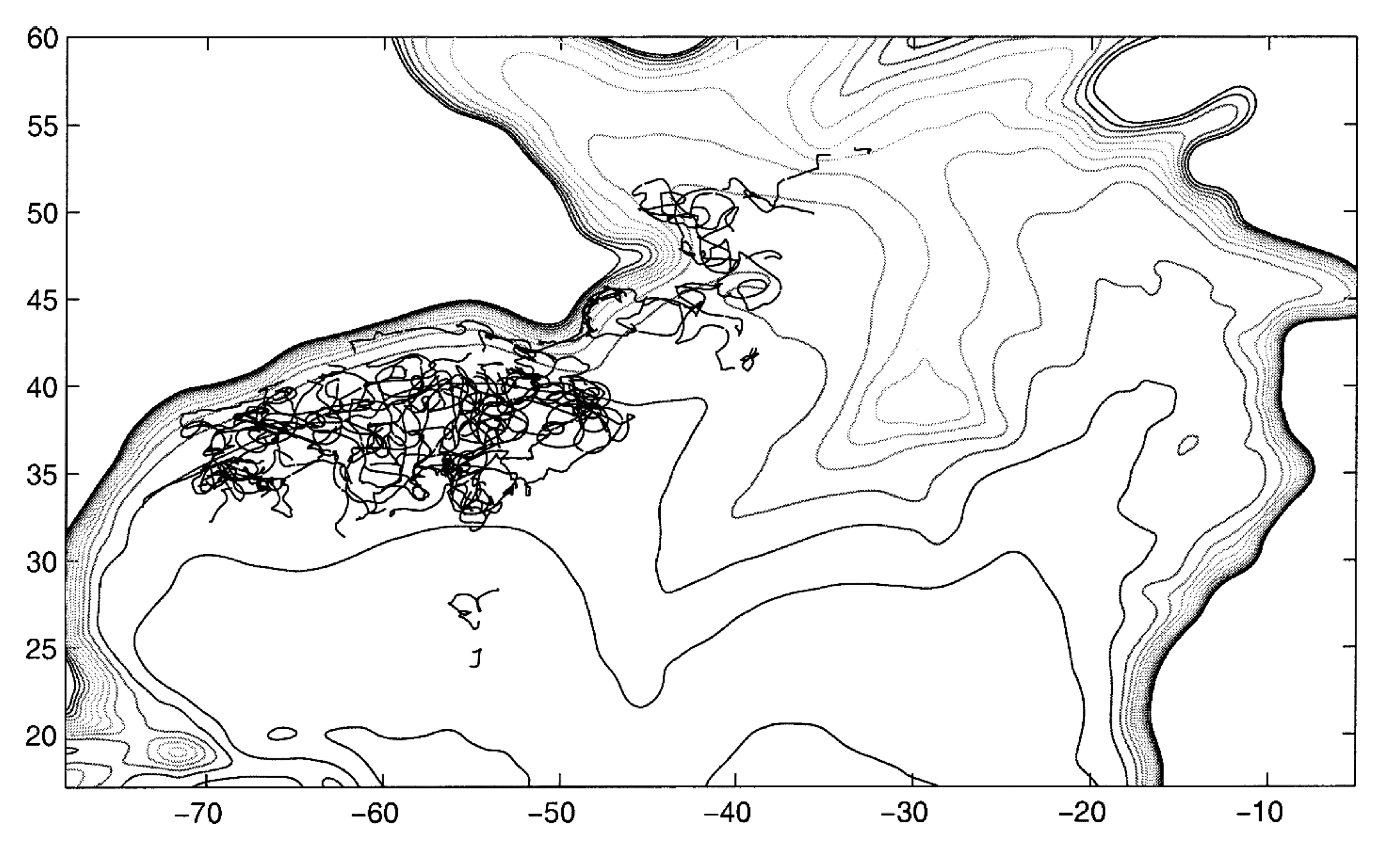
Flow Tends to be Zonal
Contours \( f/h \): combination of latitude circles and bottom topography
Over small horizontal distances, h tends to dominate,
over longer distances, the latitude-variation of f dominates.
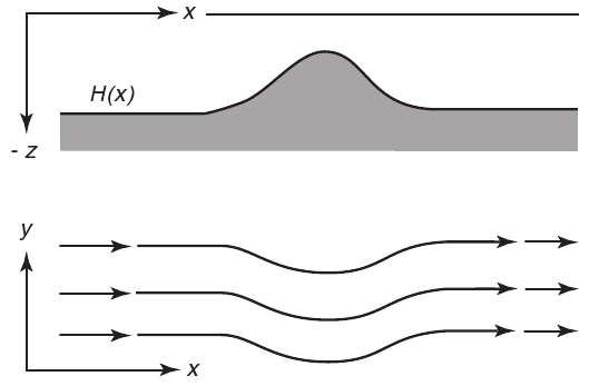
Barotropic flow over a ridge is turned equatorward
Topographic Steering at sub-sea ridge
As the depth decreases, \( \zeta+f \) must also decrease, which requires that f decrease, and the flow is turned toward the equator.
If the change in depth is sufficiently large, no change in latitude will be sufficient to conserve potential vorticity, and the flow will be unable to cross the ridge.
Dietrich et al. (1980)