Ocean Model Description
The ocean model is based on the Hamburg large-scale geostrophic
ocean model LSG (Maier-Reimer et al. 1993). The model integrates the
momentum equations, including all terms except the nonlinear advection
of momentum, by an implicit time integration method which allows a time
step of 1 month. The free surface is treated prognostically. The model
has 11 vertical levels and a horizontal resolution of 3.5![]() on a semi-staggered grid type "E" (cf. Mesinger & Arakawa 1976). A
new tracer advection scheme for temperature and salinity has been
implemented. It is an adaption of the scheme by Farrow & Stevens
(1995) using a predictor-corrector method, with a centered difference
scheme for the predictor and a third-order QUICK scheme (Leonard 1979;
Schäfer-Neth & Paul 2001) for the corrector stage. Explicit
integration of both stages results in a time step constraint that
requires the use of subcycles. Here we employ 8 subcycles, i.e. a time
step of 3.75 days for tracer advection. The QUICK scheme is less
diffusive than the standard LSG upstream scheme and less dispersive than
the common centered difference scheme.
on a semi-staggered grid type "E" (cf. Mesinger & Arakawa 1976). A
new tracer advection scheme for temperature and salinity has been
implemented. It is an adaption of the scheme by Farrow & Stevens
(1995) using a predictor-corrector method, with a centered difference
scheme for the predictor and a third-order QUICK scheme (Leonard 1979;
Schäfer-Neth & Paul 2001) for the corrector stage. Explicit
integration of both stages results in a time step constraint that
requires the use of subcycles. Here we employ 8 subcycles, i.e. a time
step of 3.75 days for tracer advection. The QUICK scheme is less
diffusive than the standard LSG upstream scheme and less dispersive than
the common centered difference scheme.
The ocean model is driven by monthly fields of wind stress, surface air temperature and freshwater flux provided by the atmospheric GCM ECHAM3/T42 (Roeckner et al. 1992). In order to close the hydrological cycle, a runoff scheme transports freshwater from the continents to the ocean. For the surface heat flux Q we use a boundary condition of the form
 |
(1) |
Influence of the surface heat flux parameters ![]() and
and ![]() on sea surface temperatures and THC stability
on sea surface temperatures and THC stability
The surface heat flux formulation (1) allows for scale selective
damping of sea surface temperature anomalies, and is therefore superior
to the conventional restoring approach. Applying ![]() W m-2 K-1 and
W m-2 K-1 and ![]() W K-1 in our model
set-up, the time scale for surface restoring can vary from one month
for small-scale temperature anomalies to almost half a year for
large-scale anomalies. It is important that these parameters allow the
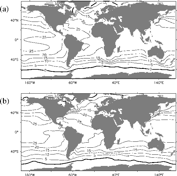
simulation of sea surface temperatures which are close to observations
(a: Model, b: Levitus observational data):
W K-1 in our model
set-up, the time scale for surface restoring can vary from one month
for small-scale temperature anomalies to almost half a year for
large-scale anomalies. It is important that these parameters allow the
simulation of sea surface temperatures which are close to observations
(a: Model, b: Levitus observational data):

It is well known that surface heat flux parameterizations have a
substantial influence on the stability properties of the THC. In
particular, a strong damping of surface temperature anomalies can
considerably decrease the stability of the "on" mode (e.g.,
Mikolajewicz & Maier-Reimer 1994; Rahmstorf & Willebrand 1995;
Lohmann et al. 1996; Prange et al. 1997). Therefore, we carried out
sensitivity experiments to demonstrate the effects of ![]() and
and ![]() on THC stability.
on THC stability.

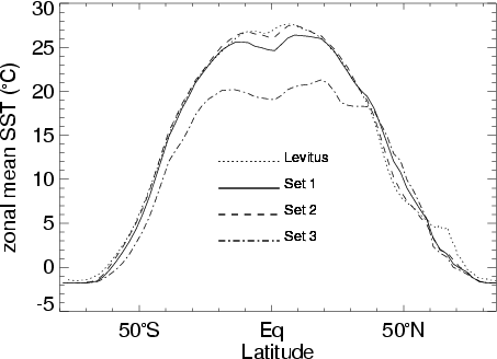
The figure above shows zonal mean sea surface temperatures using
three different sets of heat flux parameters. Standard values (see
above) are used in set 1. Set 2 defines a conventional
restoring approach, where ![]() is set to zero, and
is set to zero, and ![]() W m-2 K-1. With a
thickness of 50 m for the topmost boxes of the model grid, this
corresponds to a restoring time scale of approximately one month.
Set 3 consists of values suggested by Rahmstorf & Willebrand
(1995), i.e.
W m-2 K-1. With a
thickness of 50 m for the topmost boxes of the model grid, this
corresponds to a restoring time scale of approximately one month.
Set 3 consists of values suggested by Rahmstorf & Willebrand
(1995), i.e. ![]() W m-2 K-1
and
W m-2 K-1
and ![]() W K-1.
These authors have shown that the thermal boundary condition (1) can be
derived from an atmospheric energy balance model with diffusive lateral
heat transport. In their derivation, the restoring temperature is
strictly defined as the surface temperature that would be reached in
the absence of oceanic heat transports. Using actual air temperatures,
as we do in our set-up, the heat flux parameters of Rahmstorf &
Willebrand (1995) are not appropriate, resulting in strongly reduced
surface temperatures in low latitudes.
W K-1.
These authors have shown that the thermal boundary condition (1) can be
derived from an atmospheric energy balance model with diffusive lateral
heat transport. In their derivation, the restoring temperature is
strictly defined as the surface temperature that would be reached in
the absence of oceanic heat transports. Using actual air temperatures,
as we do in our set-up, the heat flux parameters of Rahmstorf &
Willebrand (1995) are not appropriate, resulting in strongly reduced
surface temperatures in low latitudes.
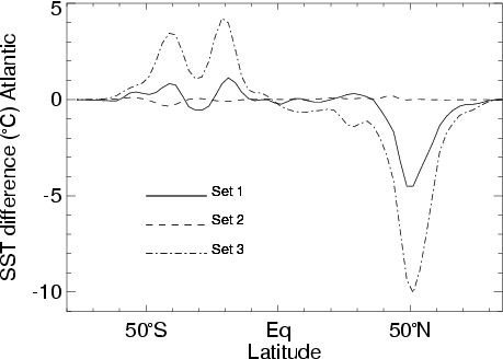
The model's capability to maintain sea surface temperature anomalies
is demonstrated in the figures below for the different sets of heat
flux parameters. Applying set 1 or set 3, we find
considerable surface temperature differences between "off" mode and
"on" mode in the North Atlantic. The strong restoring of set 2,
however, suppresses the development of temperature anomalies. North
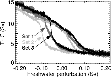
Atlantic cooling tends to stabilize the "on" mode by increasing the
density of North Atlantic water masses. This is clearly expressed in
the stability diagram.


We conclude that our standard set of parameters (![]() W m-2 K-1,
W m-2 K-1, ![]() W K-1) is a suitable
choice, allowing the simulation of observed sea surface temperatures
and the maintenance of large-scale temperature anomalies in perturbation
experiments.
W K-1) is a suitable
choice, allowing the simulation of observed sea surface temperatures
and the maintenance of large-scale temperature anomalies in perturbation
experiments.