35
Often data matrices have 2 distinct dimensions that correspond to
different physical units. For example, suppose we have
![]() representing monthly surface air temperatures along
the
representing monthly surface air temperatures along
the
35![]() N parallel at fixed spatial intervals over N/12 years.
The column M-vector
N parallel at fixed spatial intervals over N/12 years.
The column M-vector ![]() comprising all space points
at time j is
comprising all space points
at time j is ![]() 's jth column,
's jth column,
![]() for the N times. Using the
SVD representation
for the N times. Using the
SVD representation
![]() we get
the modes of
we get
the modes of ![]() ;
;
![]() 's columns are
's columns are ![]() 's EOFs, while
's EOFs, while
![]() 's columns are the corresponding `principal components'. (For
this reason, in some fields the exact same analysis is called
`principal component analysis'.) Given the above arrangement of
's columns are the corresponding `principal components'. (For
this reason, in some fields the exact same analysis is called
`principal component analysis'.) Given the above arrangement of ![]() ,
with time running along the rows and space running along the
columns (which is a very common convention),
,
with time running along the rows and space running along the
columns (which is a very common convention), ![]() 's columns span
's columns span
![]() 's column space, which corresponds to the spatial
dimension. They are
's column space, which corresponds to the spatial
dimension. They are ![]() 's EOFs. Similarly,
's EOFs. Similarly, ![]() 's columns
span
's columns
span ![]() 's row space, which corresponds to the timeseries at a
given spatial location. Because the modes are arranged in descending
order (
's row space, which corresponds to the timeseries at a
given spatial location. Because the modes are arranged in descending
order (
![]() ),
), ![]() ,
,
![]() 's 1st column,
is the spatial pattern most frequently realized, the 2nd is the
spatial pattern orthogonal to
's 1st column,
is the spatial pattern most frequently realized, the 2nd is the
spatial pattern orthogonal to ![]() 's 1st column that
is most frequently realized, and so on.
's 1st column that
is most frequently realized, and so on.
Examples will clarify matters. Consider the signal

 |
The signal is thus a linear combination of (primarily) the first rhs
term (because A's variance is 7 times larger than other additive
terms), (some of) the 2nd rhs term, and unstructured noise
![]() .
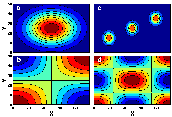
The 2 deterministic patterns are shown in
Fig.Ā1, panels b and d. Note that they are mutually
orthogonal (the cosines in both x and y are Fourier frequencies).
.
The 2 deterministic patterns are shown in
Fig.Ā1, panels b and d. Note that they are mutually
orthogonal (the cosines in both x and y are Fourier frequencies).
Now imagine 50 such f(x,y) fields (xy maps representing random
combinations of the 2 patterns plus noise as given above), or a series
of
![]() matrices
matrices
![]() .
This is
meant to simulate a geophysical situation in which a certain
time-dependent field, say sea-level pressure, is generated by some
known, deterministic, physics, plus other, low-amplitude, processes,
collectively represented here as
.
This is
meant to simulate a geophysical situation in which a certain
time-dependent field, say sea-level pressure, is generated by some
known, deterministic, physics, plus other, low-amplitude, processes,
collectively represented here as
![]() .
Given 50 realizations
of this process, we want to identify the dominant spatial patterns of
.
Given 50 realizations
of this process, we want to identify the dominant spatial patterns of
![]() ,
or, put differently, the spatial structures of
,
or, put differently, the spatial structures of ![]() that are most frequently realized.
that are most frequently realized.
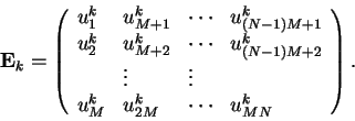
To identify these structures, we first make the 3-dimensional array
![]() (where i is the latitude
index, j is the longitude index, and k is the time index) into a
2-dimensional array (matrix), by storing an entire field in one column
vector. That is
(where i is the latitude
index, j is the longitude index, and k is the time index) into a
2-dimensional array (matrix), by storing an entire field in one column
vector. That is


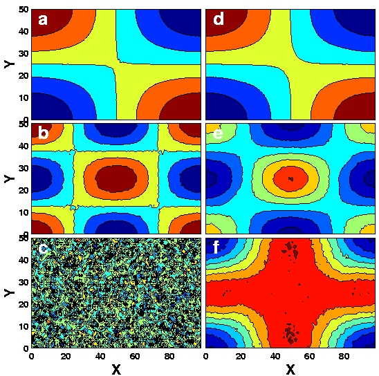 |
To demonstrate the method in action, let's use the 50 fields of the
above f(x,y,t), generated from the patterns shown in
Fig.Ā1b and d. Fig.Ā2a, b and c show the 3
leading EOFs of the cosine signal. Note how both generating patterns
are well reproduced by the method (the leading 2 patterns), despite
the noise and the random blending of the the signals by the amplitudes
A and B. Note also the sign reversal, which is completely
immaterial - the singular values (and hence the EOFs and Principal
Components) are all known to within a sign, as they are the square
root of the eigenvalues of
![]() and
and
![]() .
Clearly, the 3rd pattern, a lot like a Jackson Pollock painting,
is structureless noise.
.
Clearly, the 3rd pattern, a lot like a Jackson Pollock painting,
is structureless noise.
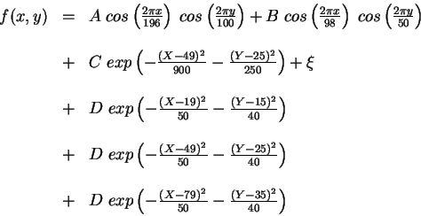
A possible critique of the previous example is that we made the method's job particularly (and artificially) easy by using 2 mutually orthogonal generating patterns. This can be fair - if the method is designed to turn arbitrary signals into an orthogonal decomposition of those signals, the real test of the method is with non-orthogonal signals.
To test this, we use the signal
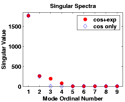 |
It is always extremely important to examine the fraction of the total variance the various modes account for. For the 2 synthetic cases above, this is shown in Fig.Ā3. (Note that only the leading 9 are shown, of of the 50 total. The rest are very near zero in both cases.) The cosine signals are very similar in both (modes 1 and 2). Higher modes differ. In the cosine only, where the only reminder is noise, it is roughly equally distributed over the entire spectrum. Conversely, in the case of the added exponentials, the remainder has 2 structured modes (the 2 exponential terms, and indeed the singular values 3 and 4 are distinct from zero. The rest, just like in the pure cosine case, are statistically indistinguishable from zero.
 |
Note that the decrease in amplitude with mode number (the falloff of the singular spectrum) is a property of the analysis, and does not always contain useful information. There is a substantial body of literature about the issue of the appropriate cutoff of the singular spectrum, beyond which, it is assumed, there is little or no useful information. The most commonly used cutoff rule in geophysics is the so-called `Rule N', which basically retains only those modes whose amplitudes stand out above the population of singular spectra extracted from a large number of synthetic matrices of the same dimensions as the one being tested. We will not treat this issue here.
 |
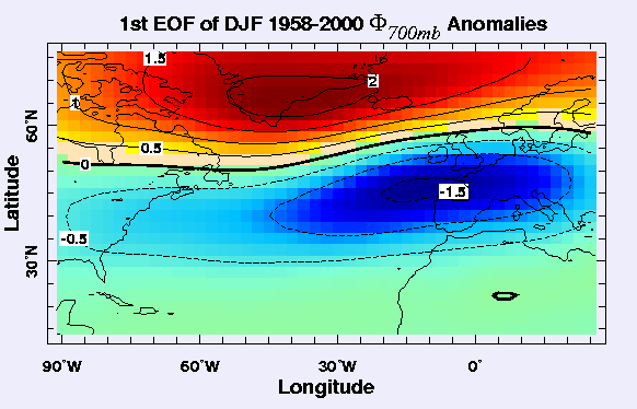
Finally, Fig.Ā4 shows an example of a real-life use of
EOFs. Height anomalies within this domain (which encompasses
![]() 5000 grid points) obviously display a very rich spectrum of
variability in time and space. And yet, when piped through the EOF
algorithm, a very clear and coherent large scale structure
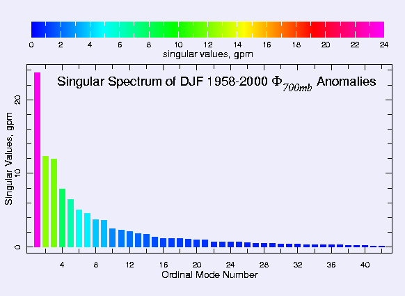
emerges. This information is corroborated by Fig.Ā5,
where the singular spectrum falloff clearly singles out the gravest
mode as substantially more important than the 2nd mode, accounting for
approximately twice as much variance.
5000 grid points) obviously display a very rich spectrum of
variability in time and space. And yet, when piped through the EOF
algorithm, a very clear and coherent large scale structure
emerges. This information is corroborated by Fig.Ā5,
where the singular spectrum falloff clearly singles out the gravest
mode as substantially more important than the 2nd mode, accounting for
approximately twice as much variance.