 |
|
By computing the EOFs and retaining a few of the first leading EOFs (
![]() ), one can compress the size of the data from
), one can compress the size of the data from
![]() to
to
![]() with a minimal loss of information (filters away much of the small-scale noise). If we have a
with a minimal loss of information (filters away much of the small-scale noise). If we have a
![]() record, such as in Fig. 8.4, stored as 100 time slices on a
record, such as in Fig. 8.4, stored as 100 time slices on a
![]() grid and we retain the 10 leading EOFs, then the data size can be
reduced from 150,000 numbers to just 16,010 numbers and still account
for about 90% of the variance in
grid and we retain the 10 leading EOFs, then the data size can be
reduced from 150,000 numbers to just 16,010 numbers and still account
for about 90% of the variance in
![]() .
.
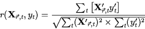
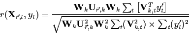
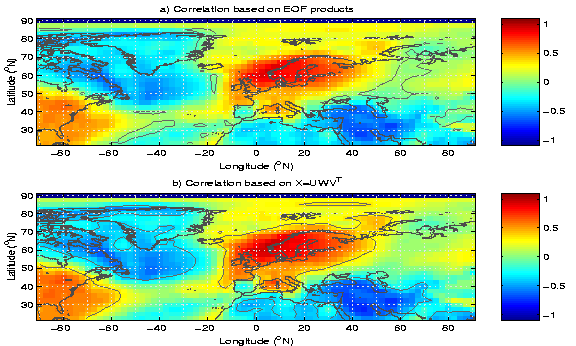
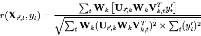
In addition to reducing the data size, the EOFs can save computation time since there are only neofs independent numbers. For instance correlation analysis can be applied to the neofs PCs, weighted by the EOF patterns and their variance, instead of the time series from
![]() points. The subscripts used below are the location vector
points. The subscripts used below are the location vector ![]() , the EOF index k and the time index t.
, the EOF index k and the time index t.
![]() is a diagonal matrix
is a diagonal matrix
The EOFs also allow better confidence limit estimates, as a confidence interval can be computed for each of the neofs PC. The geographically distributed confidence levels may be computed with a similar spatial weighting as the correlations themselves. For MC-test, using EOF products greatly reduces the computation time.
Maps of linear trends can be estimated in a simpler fashion:
![]() . The EOF products are also often used in regressional analysis and CCA.
. The EOF products are also often used in regressional analysis and CCA.