from the last lecture: Box model

for the box model at https://paleodyn.uni-bremen.de/study/Dyn2/dynamics_7_content23.html#box-model-1, you can download sevenbox_jupyter.ipynb

conda create -n jupyter-R

conda activate jupyter-R

conda install -y -c conda-forge pip notebook nb_conda_kernels jupyter_contrib_nbextensions

conda install -y -c conda-forge r r-irkernel r-ggplot2 r-dplyr

jupyter-notebook sevenbox_jupyter.ipynb

you have to download conda (or miniconda). Here a good web site: https://conda.io/projects/conda/en/latest/user-guide/install/index.html

Brownian motion, weather and climate

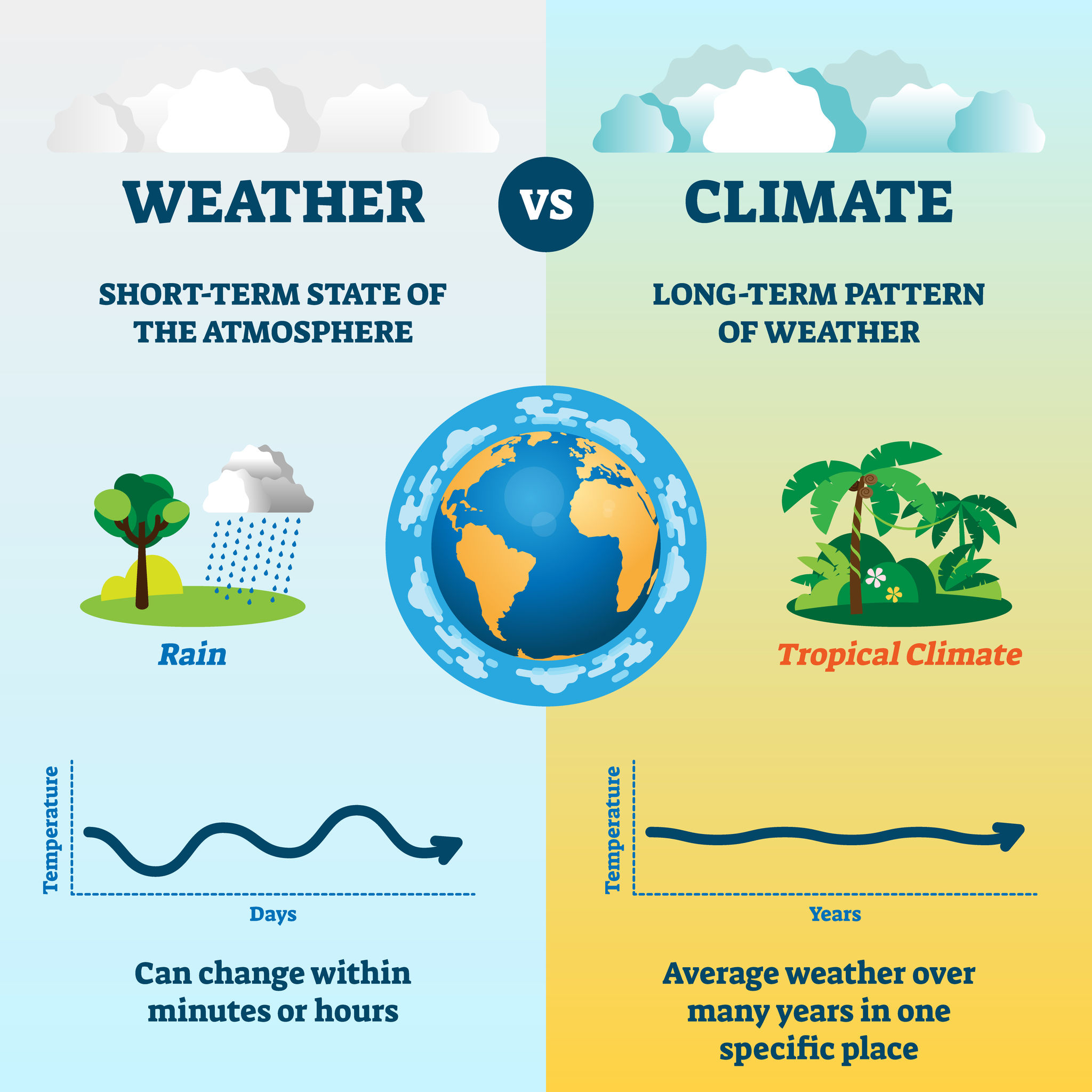
The daily observed maximum and minimum temperatures is often compared to the “normal” temperatures based upon the 30-year average. Climate averages provide a context for something like “this winter will be wetter (or drier, or colder, or warmer, etc.) than normal.

It has been said “Climate is what you expect. Weather is what you get.”

Here: general approach to the mean and fluctuations in the climate system. Indeed, the Brownian motion approach is a helpful analogue for weather and climate.

[Weather vs. Climate](http://paleodyn.uni-bremen.de/study/Dyn2/Climate-vs-weather-1.jpeg}

Difference between weather and climate?

Bundesliga

Methaphor in the football league. Predicting the outcome of the next game is difficult (weather), but predicting who will end up as German champion is unfortunately relatively easy (climate).

Physics in the 20th century

The stuff the world is made of

World views: Elementary particles, quantum mechanics, theory of relativity

Limit of divisibility (Democritus, Aristotle: Matter is not a continuous whole: “The world cannot be composed of infinitely small particles”)

Particles

Granular structure of nature

Brownian motion: displacement of particles visible under the microscope

Jerky, irregular

Brown

Molecules: disordered motion hits the particles from all directions

purely accidental

Molecules have a mass and are not infinitely small.

On the Nature of Things (ca. 60 BC)

The Roman Lucretius’s scientific poem

“You will see a multitude of tiny particles mingling in a multitude of ways… their dancing is an actual indication of underlying movements of matter that are hidden from our sight… It originates with the atoms which move of themselves”

Although the mingling motion of dust particles is caused largely by air currents, the glittering, tumbling motion of small dust particles is, indeed, caused chiefly by true Brownian dynamics.

Brownian motion

Jan Ingenhousz had described the irregular motion of coal dust particles on the surface of alcohol in 1785.

Botanist Robert Brown in 1827: studying pollen particles floating in water under the microscope. He then observed minute particles within the vacuoles of the pollen grains executing a jittery motion. By repeating the experiment with particles of dust, he was able to rule out that the motion was due to pollen particles being ‘alive’, although the origin of the motion was yet to be explained.

Mathematics of Brownian motion

Thorvald N. Thiele in 1880 in a paper on the method of least squares. This was followed independently by Louis Bachelier in 1900 “The theory of speculation”, stock and option markets.

However, it was Albert Einstein’s (in his 1905 paper) and Marian Smoluchowski’s (1906) independent research of the problem that brought the solution to the attention of physicists, and presented it as a way to indirectly confirm the existence of atoms and molecules.

The confirmation of Einstein’s theory constituted empirical progress for the kinetic theory of heat. In essence, Einstein showed that the motion can be predicted directly from the kinetic model of thermal equilibrium. The importance of the theory lay in the fact that it confirmed the kinetic theory’s account of the second law of thermodynamics as being an essentially statistical law.

Diffusion of Brownian particles

Diffusion_of_Brownian_particles

The characteristic bell-shaped curves of the diffusion of Brownian particles. The distribution begins as a Dirac delta function, indicating that all the particles are located at the origin at time t=0, and for increasing times they become flatter and flatter until the distribution becomes uniform in the asymptotic time limit.

Diffusion of Brownian particles

\[ \rho(x, t+\tau) = \rho(x, t) \cdot 1 + 0 + \frac{\partial^2 \rho}{\partial x^2} \cdot \int_{-\infty}^{+\infty} \frac{\Delta^2}{2} \cdot \phi(\Delta) \, \mathrm{d} \Delta \quad + \quad ... \]

The integral in the first term is equal to one by the definition of probability, and the second and other even terms (i.e. first and other odd moments) vanish because of space symmetry.

\[ \frac{\partial\rho}{\partial t} = \frac{\partial^2 \rho}{\partial x^2} \cdot \int_{-\infty}^{+\infty} \frac{\Delta^2}{2\, \tau} \cdot \phi(\Delta) \, \mathrm{d} \Delta + \mathrm{higher\;order\; even\; moments} \]

Where the second moment of probability of displacement \(\Delta,\) is interpreted as diffusivity \[ D = \int \frac{\Delta^2}{2\, \tau} \cdot \phi(\Delta) \, \mathrm{d} \Delta \]

Then the density of Brownian particles \(\rho\) at point x at time t satisfies the diffusion equation: \[ \frac{\partial\rho}{\partial t}=D\cdot \frac{\partial^2\rho}{\partial x^2} \]

Einstein’s paper

Diffusion_of_Brownian_particles

Einstein’s formula 1905

Diffusion_of_Brownian_particles

Mean squared displacement

Density of Brownian particles \(\rho\) satisfies the diffusion equation: \[ \frac{\partial\rho}{\partial t}=D\cdot \frac{\partial^2\rho}{\partial x^2} \]

Assuming that N particles start from the origin at the initial time \[ \rho(x,t)=\frac{N}{\sqrt{4\pi Dt}}e^{-\frac{x^2}{4Dt}}. \]

This expression allowed Einstein to calculate the moments directly. The first moment is seen to vanish, meaning that the Brownian particle is equally likely to move to the left as it is to move to the right. The second moment is, however, non-vanishing, being given by

\[ \overline{x^2}=2\,D\,t. \]

This expresses the mean squared displacement in terms of the time elapsed and the diffusivity. From this expression Einstein argued that the displacement of a Brownian particle is not proportional to the elapsed time, but rather to its square root.

Diffusion of Brownian particles

left: 20%

Nparticle<-1000 #number of particles
T<-  1000   #integration time in time units
h<-  0.5   #step size in time units
beta<-0.00001 #friction term
lambda<-1 #noise term
N<-T/h
t<-(0:(N-1))*h

x<-matrix(0,Nparticle,N) # Initial condition, all = 0

for (i in 1:(N-1)) 
{x[,i+1]<-x[,i]*(1-beta*h)+ rnorm(Nparticle)*sqrt(h)}

plot(0,xlim=c(0,T),ylim=c(-100,100),type="n")
for (i in 1:N) lines (t,x[i,],col=i)

#analyse the densities
h<-matrix(0,N,40)

for (i in 1:(N-1)) h[i,]<-hist(x[,i],breaks=c((-20:20)*10),freq=FALSE,ylim=c(0,0.04))$counts

filled.contour(t,(-19:20)*10-5,h,color.palette=rainbow,xlab="time",ylab="space")

stochastic differential equation

In a stochastic framework of climate theory \[ \frac{d}{dt} x(t) = f(x) + g(x) \xi , \] where \(\xi\) is a stationary stochastic process and the functions f, g describe the climate dynamics. The properties of the random force are described through its distribution and its correlation properties at different times.

The process \(\xi\) is assumed to have a Gaussian distribution of zero average, \[ < \xi (t) > = 0 \] and to be \(\delta\)-correlated in time, \[ < \xi(t) \xi(t +\tau) > = \delta (\tau) \label{deltacorr} \] where \(\delta\) is the delta function defined by \[ \int f (x) \, \delta (x-x_0) \, dx = f(x_0) \quad . \]

The brackets indicate an average over realizations of the random force.

stochastic differential equation …

Using the ergodic hypothesis, the ensemble average
\[ \left\langle \qquad \right\rangle \]

can be expressed as the time average \[ \quad \lim_{T \to \infty} \frac{1}{T} \int_{-T/2}^{T/2} dt \]

For a Gaussian process only the average and second moment need to be specified since all higher moments can be expressed in terms of the first two. Note that the dependence of the correlation function on the time difference \(\tau\) assumes that \(\xi\) is a stationary process.

Imagine a so-called red-noise process \[ \frac{dx}{dt} = -\lambda x + \xi \, \]

Climate System

climate

Probability

climate

Stochastic climate model

Imagine that the temperature of the ocean mixed layer of depth \(h\) is governed by \[ \frac{dT}{dt} = -\lambda T + Q \, , \] where \(\lambda\) is the typical damping rate of a temperature anomaly, and Q is the air-sea fluxes due to weather systems are represented by a white-noise process with zero average \[< Q_{} > = 0 \]

and \(\delta\)-correlated in time

\[ Cov_Q(\tau)= < Q_{}(t) Q_{}(t +\tau) > = c \cdot \delta (\tau) \]

The Fourier transform of the auto-correlation function \(Cov_Q (\tau)\) is called spectrum \[ S_Q(\omega) = \int Cov_Q (\tau) e^{i \omega \tau} \, d\tau \quad = \int c \cdot \delta (\tau) e^{i \omega \tau} \, d\tau \quad = \quad c \]

Remember: \[ x (t) = \frac{1}{2 \pi} \int \hat x(\omega) e^{-i \omega t} \, d\omega \quad \]

Solve the temperature response \(T= \hat{T}({\omega}) e^{-i\omega t}\) and hence show that:

\[ \hat{T} ({\omega}) = \frac{\hat{Q}({\omega})}{\left({\lambda}-i \omega\right)} \]

It is helpful to look onto the Fourier transformation. \[ Q_{} = \frac{1}{2 \pi} \int \hat{Q}({\omega}) e^{-i\omega t} \, d\omega \quad \] where \(\hat{Q}({\omega})\) is the amplitude of the random forcing at frequency \(\omega\).

2. Show that it has a spectral density \(\hat{T}({\omega}) \, \hat{T}^{*}({\omega})\) is given by: \[ \hat{T} \, \hat{T}^{*}= \frac{\hat{Q} \, \hat{Q}^{*}}{\left({\lambda}^{2}+ \omega^{2}\right)} \] where \(\hat{Q}^{*}\) is the complex conjugate.

3. Show that the spectrum of T is

\[ S_T(\omega) = <\hat{T} \, \hat{T}^{*}> = \frac{< \hat{Q} \, \hat{Q}^{*}>}{\left({\lambda}^{2}+ \omega^{2}\right)}= \frac{c}{\left({\lambda}^{2}+ \omega^{2}\right)}. \]

The brackets \(< \dots >\) denote the ensemble mean. Make a sketch of the spectrum \(S_T\) using a log-log plot. Why is it called red noise?

Fluctuations with a frequency greater than \({\lambda}\) are damped.