Dynamics II: Sheet 5

Lecture: May 23 (Monday), 14:00 Prof. Dr. Gerrit Lohmann

Tutorial: May 23 (Monday), 16-17; Smit Doshi, Dr. Qiyun Ma

 
 

Preparation

 

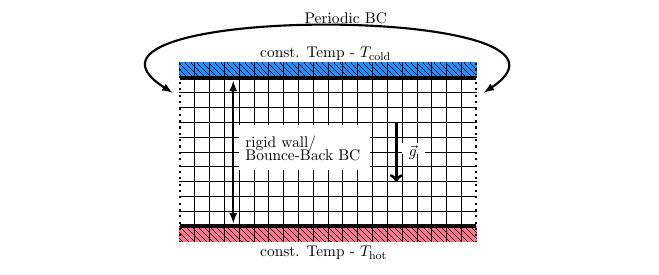
Rayleigh-Bénard convection and bifurcation

Experiments:

trailer Cellules de Bénard (1min),
Rayleigh–Bénard convection made with mix of cooking oil and small aluminium particles (5 min),
Was haben Benard-Zellen mit Kochen zu tun? (3 min, German)

Simulations:

Rayleigh Benard Thermal Convection with LBM (5 min),
Rayleigh Benard Thermal Convection 3D Simulation (2 min)
Sketch,
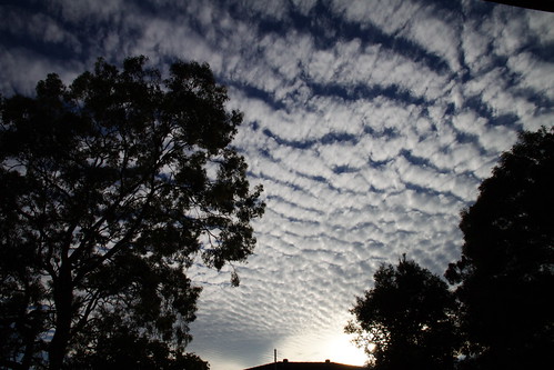
Clouds,
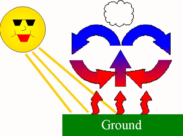
Cartoon

Bifurcations

Bifurcation youtube (20 min)
Bifurcation Khan academy (13 min) Reading Bifurcation theory

 
 

Lecture

 

Content in the script: Rayleigh-Bénard convection, Lorenz system, nonlinear dynamics, bifurcations, multiple equilibria

 

Exercise 4 introduced, questions to the exercise (15 min)

 

Homework 1: Solve Exercise 4

 

 

Lorenz model

r=24
s=10
b=8/3
dt=0.01
x=0.1
y=0.1
z=0.1
vx<-c(0)
vy<-c(0)
vz<-c(0)
for(i in 1:10000){
x1=x+s*(y-x)*dt
y1=y+(r*x-y-x*z)*dt
z1=z+(x*y-b*z)*dt
vx[i]=x1
vy[i]=y1
vz[i]=z1
x=x1
y=y1
z=z1
}
plot(vx,vy,type="l",xlab="x",ylab="y",main="LORENZ ATTRACTOR")

r=5000/150000
#r=1/10
Bev=85000000
K=1
dt=0.01

N=150000/Bev

vN=c(0); vNp=c(0); vt=c(0)
vN[1]=N; vNp[1]=0; vt[1]=0

for(i in 2:100000){
N1=N+r*N*(1-N/K)*dt
vNp[i]=r*N*(1-N/K)
vN[i]=N1
vt[i]=i*dt
N=N1
}

plot(vt,vN,type="l",xlab="time [days]",ylab=" ",main="Logistic growth Corona: N(t)", lwd=2, lty="solid", cex.main=3, cex.lab=3, cex.axis=3,cex.lab=3)

plot(vt,vNp*Bev/100,type="l",xlab="time [days]",ylab=" ",main="New infections/100: intensive care medicine",cex.main=3, cex.lab=3,cex.axis=3,cex.lab=3)

max(vNp[]*Bev/100)

## [1] 7083.333