Dynamics II: lecture 2
Gerrit Lohmann date: April 19, 2021
Summary of last lecture
Non-dimensional parameters: Reynolds number
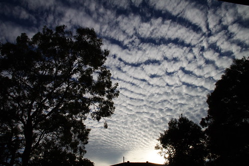
Preparation: Videos Rayleigh-Benard convection
Experiments:
trailer Cellules de Bénard (1min), Rayleigh–Bénard convection: cooking oil and small aluminium particles (5 min), Was haben Benard-Zellen mit Kochen zu tun? (3 min, German)
Simulations:
Rayleigh Benard Thermal
Convection with LBM (5 min),
Rayleigh Benard Thermal
Convection 3D Simulation (2 min)
 sketch
Mathematical concept of bifurcation: Instability
Bifurcation youtube,
Bifurcation Khan academy,
Bifurcation K
Max and Moritz, not lazy,
sawing secretly a gap in the bridge.
When now this act is over, you suddenly hear a scream:
“Hey, out! You billy goat!
Tailor, tailor, bitch, bitch, bitch!”
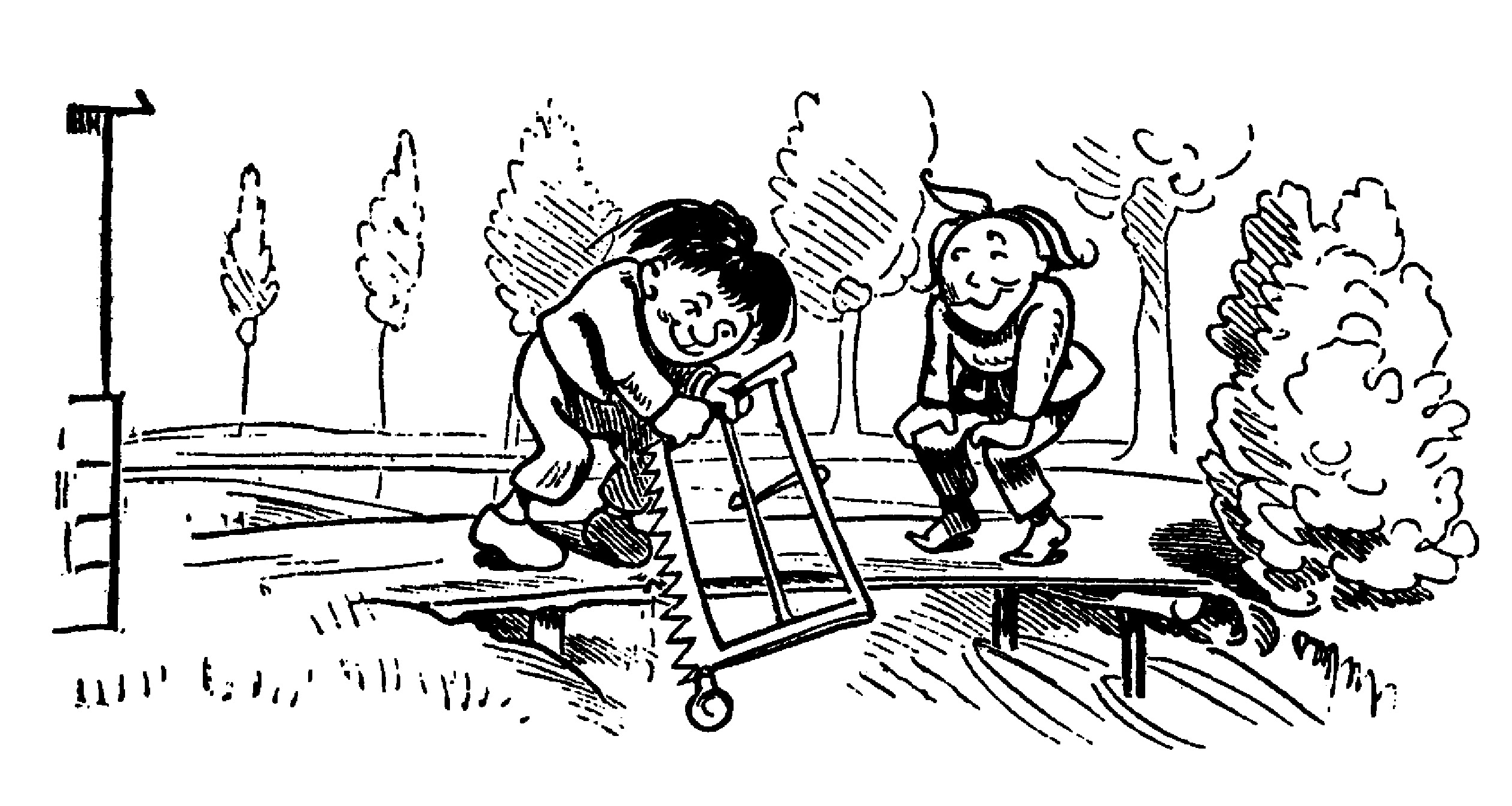
Stability - Instability: Tailor Böck
And there he is on the bridge,
Cracks! The bridge is falling apart;
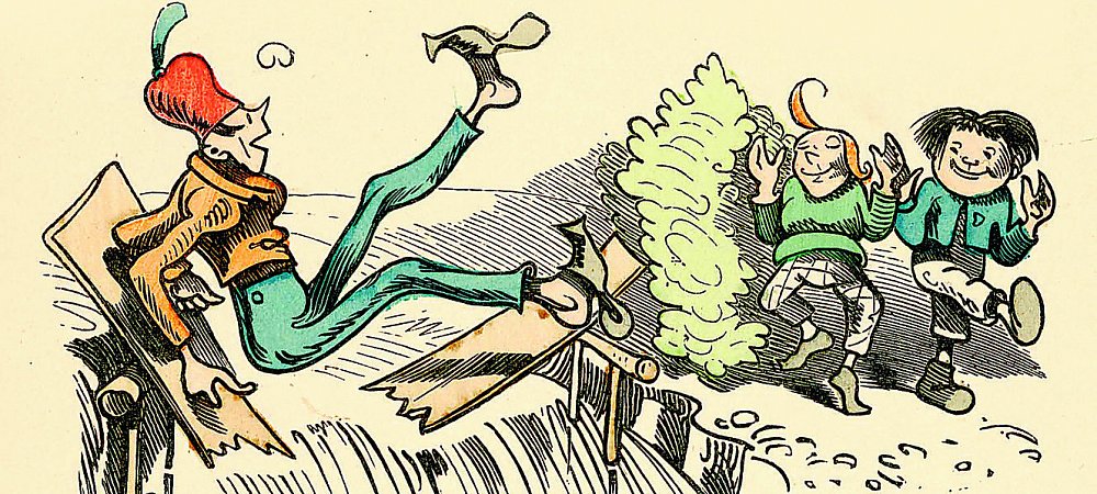
Schneider Böck has a fast stream flowing in front of his house. M & M taunt him by making goat noises, until he runs outside. The bridge breaks; the tailor is swept away and nearly drowns (but for two geese, which he grabs a hold of).
Stability - Instability
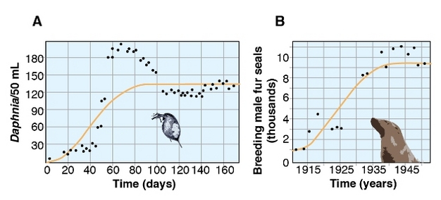
Verhulst: Self-limiting growth
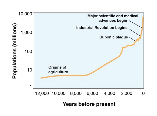
Human population: logistic growth model
Coronavirus epidemic: logistic growth model
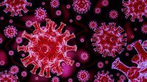
N is the number of cases,
r infection rate,
p cure rate,
K final epidemic size.
dN/dt linearly decreases with the number of cases.
Coronavirus epidemic: logistic growth model
r=2000/150000


[1] 2833.333
r=5000/150000


[1] 7083.333
Organization of
Linear stability analysis
Linear stability analysis
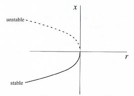
Saddle-node bifurcation: two fixed points collide
The normal form: \[ \frac{dx}{dt}=b+x^2 \]
\[ b<0: \mbox{ a stable equilibrium point at } -\sqrt{-b} \mbox{ and an unstable one at } \sqrt{-b} \qquad \qquad \]
\( b=0 \): exactly one equilibrium point, saddle-node fixed point.
\( b>0 \): no equilibrium points. Saddle-node bifurcations may be associated with hysteresis loops.
Saddle-node bifurcation: two fixed points collide
Saddle-node bifurcation: two fixed points collide
3) Potential or Lyapunov Method
\[ \frac{dx}{dt}=b+x^2 = - \frac{d}{dx} \left( - b x - \frac{x^3}{3} \right) = - \frac{d}{dx} V (x) \]

Global analysis including basins of attraction for \( x_{E2}: (-\infty,3) \)
4) Graphical method: slope at equilibrium points
\[ \frac{dx}{dt}=b+x^2 \]
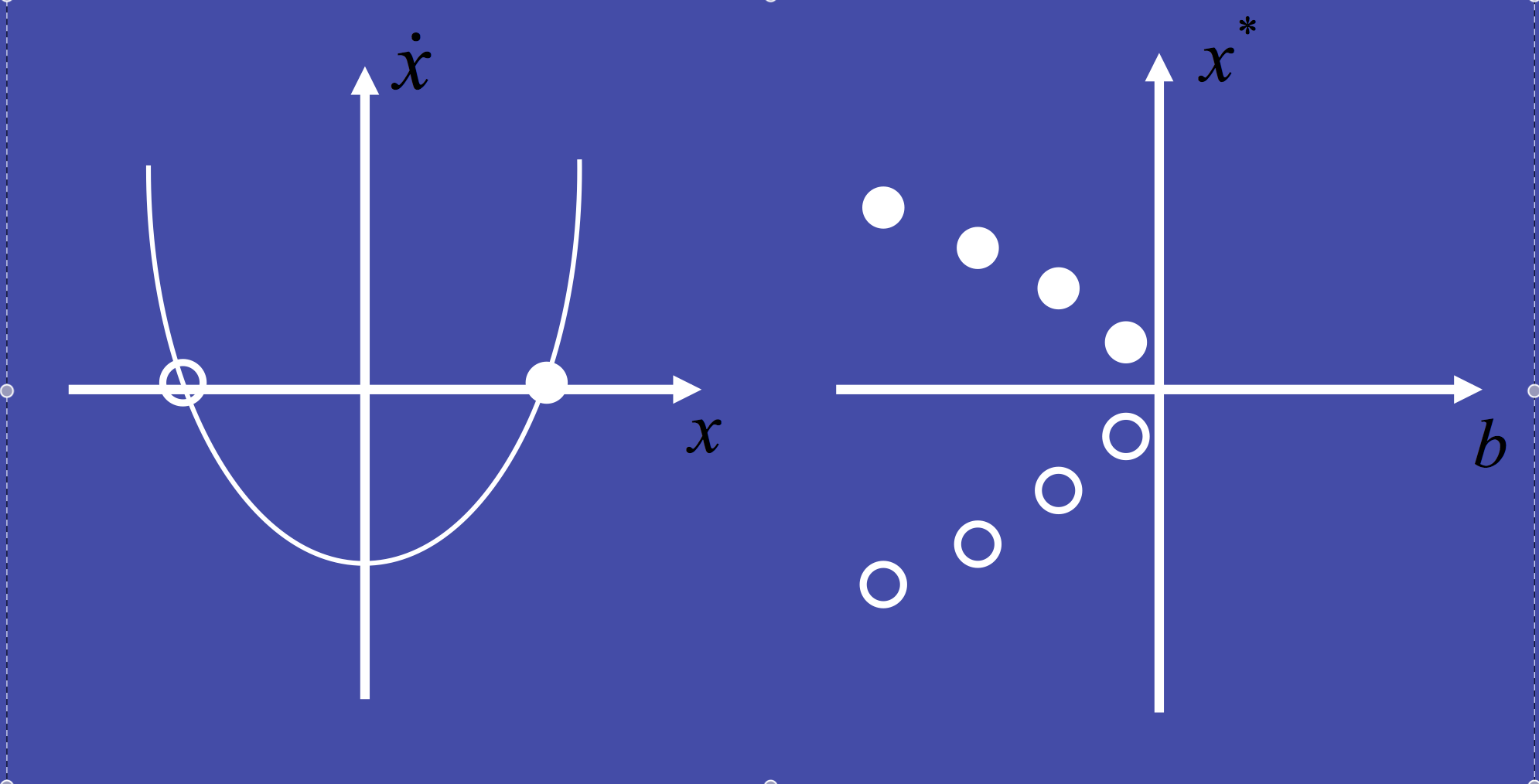
filled points: positive slope => unstable
open points: negative slope => stable
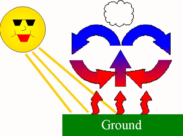
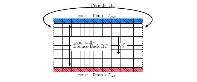
Convection in the Rayleigh-Benard system
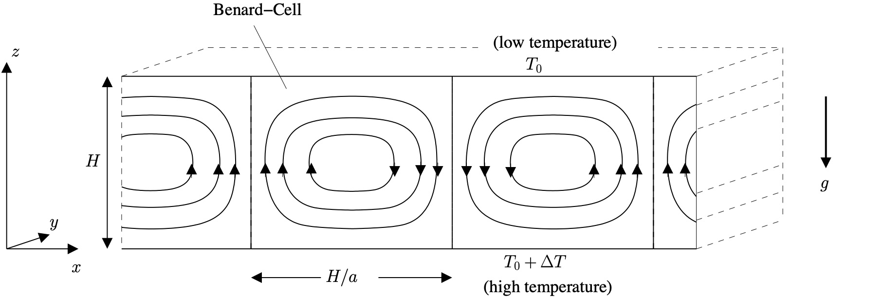
Rayleigh (1916) temperature difference between the upper- and lower-surfaces \[ T(x, y, z=H) = \, T_0 \] \[ T(x, y, z=0) \, = \, T_0 + \Delta T \]
Furthermore \[ \rho = \rho_0 = const. \] except in the buoyancy term, where:
\[ \varrho = \varrho_0 (1 - \alpha(T-T_0)) \mbox{ with } \alpha > 0 \quad . \]
common feature of geophysical flows
No Convection Equilibrium: Diffusion
Diffusion: Temperature varies linearly with depth:
\[ T_{eq} = T_0 + \left(1 - \frac{z}{H}\right) \Delta T \]
No movement of particles:
\[ u = w= 0 \]
When this solution becomes unstable, convection should develop.
Vorticity in the Rayleigh-Benard system
Temperature in the Rayleigh-Benard system
Temperature in the Rayleigh-Benard system
Non-dimensional Rayleigh-Benard system
Non-dimensional Rayleigh-Benard system
Non-dimensional Rayleigh-Benard system
Galerkin approximation: Get a low-order model
Rayleigh number Ra: Buoyancy & Viscosity
\[ \mbox{Motion develops if } \quad R_a = \frac{g \alpha H^3 \Delta T}{\nu \kappa} \quad \mbox{exceeds } \quad R_c = \pi^4 \frac{(1+a^2)^3}{a^2} \]
\[ \mbox{The minimum value of $R_c = 657.51$ occurs when $a^2 = 1/2$. } \]
\[ \mbox{When } R_a < R_c,\mbox{ heat transfer is due to conduction} \]
\[ \mbox{When } R_a > R_c, \mbox{ heat transfer is due to convection.} \]
Lorenz system
Lorenz system r=24


Lorenz system r=0.9


Lorenz system r=3.5

