Dynamics II: lecture 4
Gerrit Lohmann date: May 3, 2021
Organization of
Scaling of the momentum
In the coordinate system
Example: Vorticity for a rigid body
\[ \nabla \times \boldsymbol{ u} = 2 \boldsymbol{ \Omega} \]
Example: Vorticity from shear at Cape Haterras
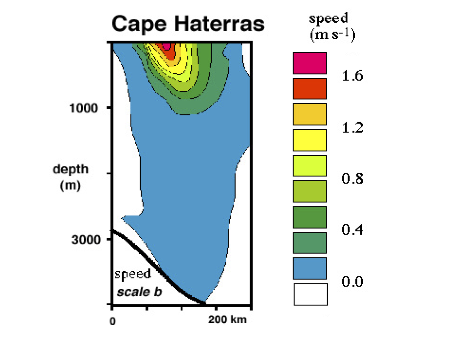
Tomczak & Godfrey
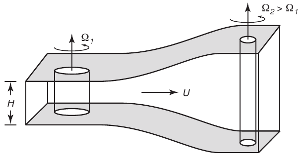
Potential vorticity is conserved
\[ \frac{D}{Dt}\left(\zeta+f\right) + \left(\zeta + f\right)\left(\frac{\partial u}{\partial x}+\frac{\partial v}{\partial y}\right)=0 \quad \]
Couples depth, vorticity, latitude
– Changes in the depth results in change in \( \zeta \).
– Changes in latitude require a corresponding change in \( \zeta \).
Dietrich et al. (1980)
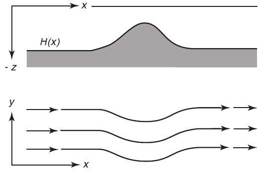
Ocean with depth h(x,y)
\[ \frac{D}{Dt}\left( \frac{\zeta+f}{h}\right) = 0 \quad \]
Steward, Oceanography
Conservation of Vorticity
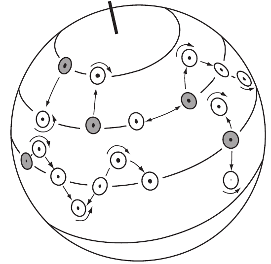
Vorticity tends to be conserved as columns of water change latitude. After von Arx (1962).
Taylor-Proudman Theorem
\[ \mbox{Assume constant density } \rho_0 \mbox{ on a plane with constant rotation } f=f_0 \neq 0 \]
\[ \frac{\partial v}{\partial z}=\frac{\partial u}{\partial z}=\frac{\partial v}{\partial z}=0 \]
Flow is two-dimensional and does not vary in the vertical direction.
Theorem applies to slowly varying flows.
Physical origin: stiffness endowed to the fluid by rapid rotation of the Earth.
Taylor's lab experiments: homogeneous fluid tends to move in vertical columns
Vertical velocity & north-south currents
Vertical velocity & north-south currents
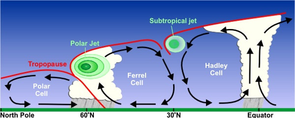
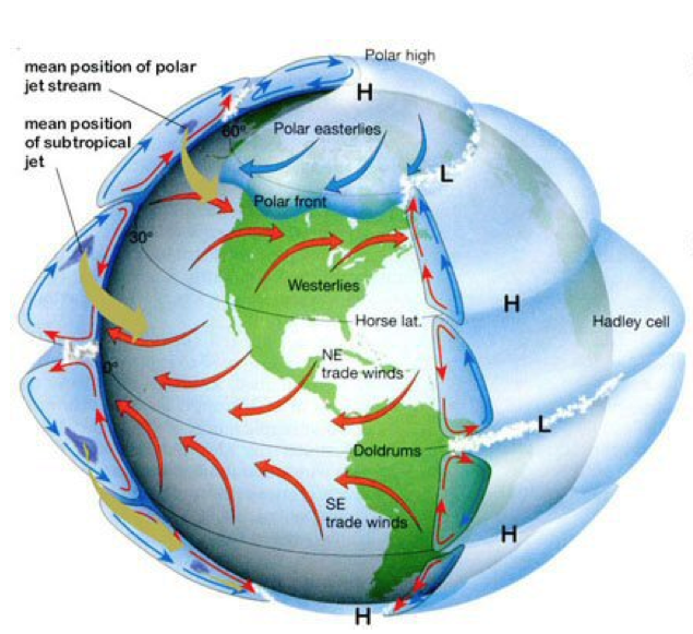
Angular Momentum and Hadley Cell
Angular Momentum
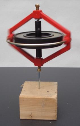
Gyroscope remains upright while spinning due to conservation of its angular momentum
Angular Momentum and Hadley Cell
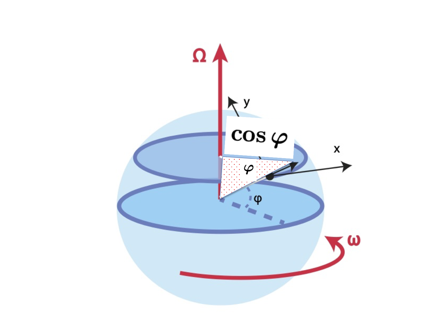
\( \Omega \) Earth rotation rate, \( u \) eastward wind
\( R= a \cos \varphi \) distance from rotation axis
\( U = R \Omega \) solid body speed
Angular Momentum and Hadley Cell
\( \Omega \) Earth rotation rate, \( u \) eastward wind
\( R= a \cos \varphi \) distance from rotation axis
\( U = R \Omega R \) solid body speed
Angular Momentum and Hadley Cell
Angular Momentum and Hadley Cell
Angular Momentum and Hadley Cell
Angular Momentum and Hadley Cell
a) Conservation of A, u-equation of motion
a) Conservation of A, u-equation of motion
b) Conservation of A explains subtropical jet
\[ \mbox{At the equator } A_0 = \Omega a^2, \mbox{ flow rises from the ground there with no relative motion } \]
We have \[ A = \Omega a^{2} \cos^{2} \varphi + u a \cos \varphi = A_0 = \Omega a^2 \]
\[ u a \cos \varphi = \Omega a^2 ( 1 - \cos^{2} \varphi ) \]
\[ u = \Omega a \frac{\sin^2 \varphi}{ \cos \varphi } \]
The zonal flow u will be greatest at the edge of the cell, where \( \varphi \) is greatest, thus producing the subtropical jet.
b) Conservation of A explains subtropical jet
Assume the Hadley circulation is symmetric about the equator, and its edge is at 20°N, determine the strength of the subtropical jet by \[ u (20^\circ) = \Omega a \sin^{2} (20^\circ) / \cos (20^\circ) \, = \, \, \, 57.6 \, m \, s^{-1} \]
(The observed zonal winds are weaker than the value. In reality, non-axisymmetric atmospheric eddies act to reduce angular momentum strength of the jet.)
Solution c) about low-level return flow
Solution c) about low-level return flow
d) Hadley Circulation in northern winter
d) Hadley Circulation in northern winter
Engery balance model
What drives the ocean currents?
What drives the ocean currents?
Sverdrup relation
Sverdrup relation
Sverdrup relation
Sverdrup transport
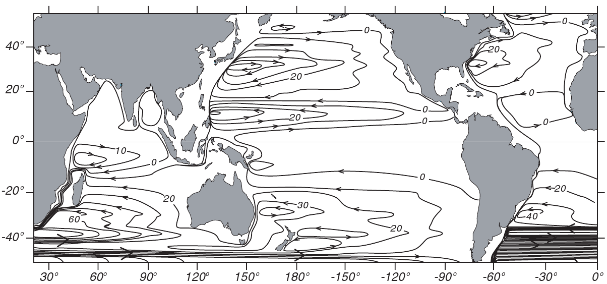
applied globally using the wind stress from Hellerman and Rosenstein (1983). Contour interval is \( 10 \) Sverdrups (Tomczak and Godfrey, 1994).
\[ V = \frac{1}{\rho \beta} \, \left( \frac{\partial \tau_{yz} }{\partial x} \, - \frac{\partial \tau_{xz}}{\partial y}\, \right) = \frac{1}{\rho \beta} \, \, \operatorname{curl} \, \tau \]
Ekman Pumping in a thin Ekman layer
Ekman Pumping in a thin Ekman layer
Ekman Pumping in a thin Ekman layer
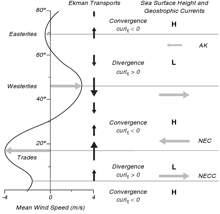
Ekman Pumping & Sverdrup Transport
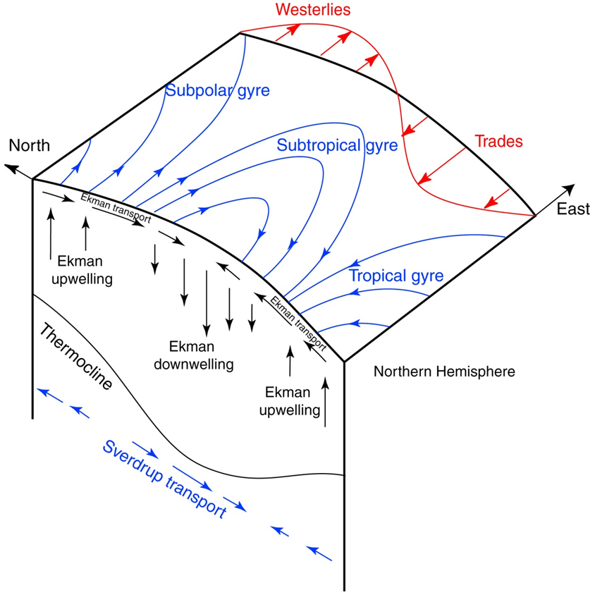
Ekman vertical & vertical geostrophic velocities
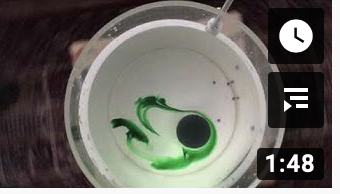
Tea leaf paradox: Friction on the bottom matters
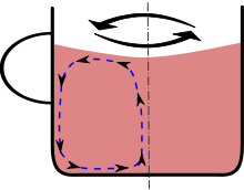
Tea leaf paradox: Friction on the bottom matters
Low Pressure: Friction on the bottom matters
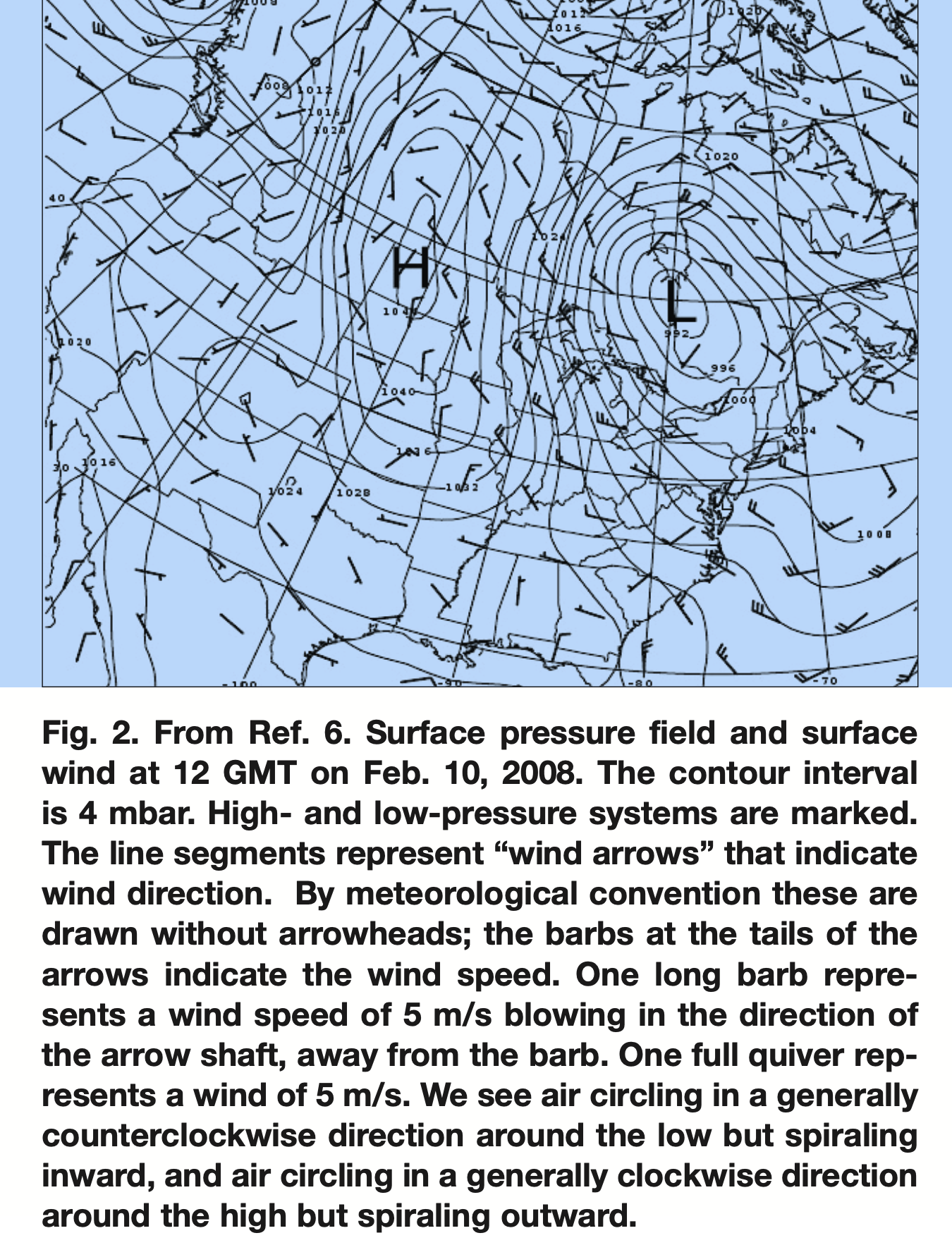
Low Pressure: Friction on the bottom matters