Dynamics II
Lecture: June 5, 2023 (Monday), 14:00 Prof. Dr. Gerrit Lohmann
Overview of Dynamics II
Solution of Temperature Advection
The total change of temperature is given by \[ \frac{d T}{dt} = \frac{\partial T}{\partial t} + {\bf u} \cdot \nabla T = \dot{q} \] \[ \Leftrightarrow \quad \frac{\partial T}{\partial t} = - {\bf u} \cdot \nabla T + \dot{q} \] Here we use the velocity \[ {\bf u} = - 20 \frac{m}{s} \cdot \frac{1}{\sqrt{2}} (1, 1, 0) , \qquad \nabla T = \frac{{3}{^\circ C}}{{50}{km}} (0, -1, 0), \qquad \dot{q} = 1 \frac{^\circ C}{h} \] Then we calculate the temperature change at the station \[ \frac{\partial T}{\partial t} = - {\bf u} \cdot \nabla T + \dot{q} \]
\[ \frac{\partial T}{\partial t} = 20 \frac{m}{s} \, \frac{1}{\sqrt{2}} (1, 1, 0) \cdot (0, -1, 0) \frac{{3}{^\circ C}}{{50}{km}} + 1 \frac{^\circ C}{h} \approx {-2.1} \frac{^\circ C}{h} \]
Elimination of the pressure term
in the 2D-Navier-Stokes equation.
2D: assume \(w = 0\) and no dependence of anything on z
\[ \rho \left(\frac{\partial u}{\partial t} + u \frac{\partial u}{\partial x} + v \frac{\partial u}{\partial y}\right) = -\frac{\partial p}{\partial x} + \mu \left(\frac{\partial^2 u}{\partial x^2} + \frac{\partial^2 u}{\partial y^2}\right) \] \[ \rho \left(\frac{\partial v}{\partial t} + u \frac{\partial v}{\partial x} + v \frac{\partial v}{\partial y}\right) = -\frac{\partial p}{\partial y} + \mu \left(\frac{\partial^2 v}{\partial x^2} + \frac{\partial^2 v}{\partial y^2}\right) \]
Procedure
Differentiating the first with respect to y: \[\partial_y\]
the second with respect to x: \[\partial_x\]
and subtracting the resulting equations will eliminate pressure and any potential force.
Defining the stream function \(\psi\) through \[ u = \frac{\partial \psi}{\partial y} \quad ; \quad v = -\frac{\partial \psi}{\partial x} \]
results in mass continuity being unconditionally satisfied (given the stream function is continuous), and then incompressible Newtonian 2D momentum and mass conservation degrade into one equation:
\[ \frac{\partial}{\partial t}\left(\nabla^2 \psi\right) + \frac{\partial \psi}{\partial y} \frac{\partial}{\partial x}\left(\nabla^2 \psi\right) - \frac{\partial \psi}{\partial x} \frac{\partial}{\partial y}\left(\nabla^2 \psi\right) = \nu \nabla^4 \psi \]
or using the total derivative\[ D_t \left(\nabla^2 \psi\right) = \nu \nabla^4 \psi \] \(\nabla^4\) is the (2D) biharmonic operator and \(\nu\) the kinematic viscosity \(\nu=\frac{\mu}{\rho}.\)
This single equation describes 2D fluid flow, kinematic viscosity as parameter!
The concept will become very important in ocean dynamics. The term \[\zeta=\nabla^2 \psi\]
is called relative vorticity, its dynamics can be described as \[ D_t \zeta = \nu \nabla^2 \zeta \quad \]
Non-dimensional parameters: The Reynolds number
For the case of an incompressible flow in the Navier-Stokes equations, assuming the temperature effects are negligible and external forces are neglected.
conservation of mass \[ \nabla \cdot \mathbf{u} = 0 \] conservation of momentum \[ \partial_t \mathbf{u} + ( \mathbf{u} \cdot \nabla) \mathbf{u} = - \frac{1}{\rho_0} \nabla p + \nu \nabla^2 \mathbf{u} \]
The equations can be made dimensionless by a length-scale L, determined by the geometry of the flow, and by a characteristic velocity U.
For analytical solutions, numerical results, and experimental measurements, it is useful to report the results in a dimensionless system (concept of dynamic similarity).
Goal: replace physical parameters with dimensionless numbers, which completely determine the dynamical behavior
representative values for velocity \((U),\) time \((T),\) distances \((L)\)
Using these values, the values in the dimensionless-system (written with subscript d) can be defined: \[ u =U \cdot u_d \] \[ t = T \cdot t_d \] \[ x = L \cdot x_d \] with \(U = L/T\).
From these scalings, we can also derive \[ \partial_t = \frac{\partial}{\partial t } = \frac{1}{T} \cdot \frac{\partial}{\partial t_d } \] \[ \partial_x = \frac{\partial}{\partial x} = \frac{1}{L} \cdot \frac{\partial}{\partial x_d } \] Note furthermore the units of \([\rho_0] = kg/m^3\), \([p] = kg/(m s^2)\), and \([p]/[\rho_0]= m^2/s^2\). Therefore the pressure gradient term has the scaling \(U^2/L\).
\[ \nabla_d \cdot \mathbf{u_d} = 0 \] and conservation of momentum
…
The dimensionless parameter \[ Re=UL/ \nu \]
is the Reynolds number and the only parameter left!
For large Reynolds numbers, the flow is turbulent.
In most practical flows \(Re\) is rather large \((10^4-10^8),\) large enough for the flow to be turbulent. A large Reynolds number allows the flow to develop steep gradients locally.
In the literature, the term “equations have been made dimensionless”, means that this procedure is applied and the subscripts d are dropped.
Rayleigh-Benard convection (and Rayleigh number)
Experiments:
Rayleigh–Bénard convection: cooking oil and small aluminium particles (5 min),
Rayleigh Benard
Thermal Convection 3D Simulation (2 min)

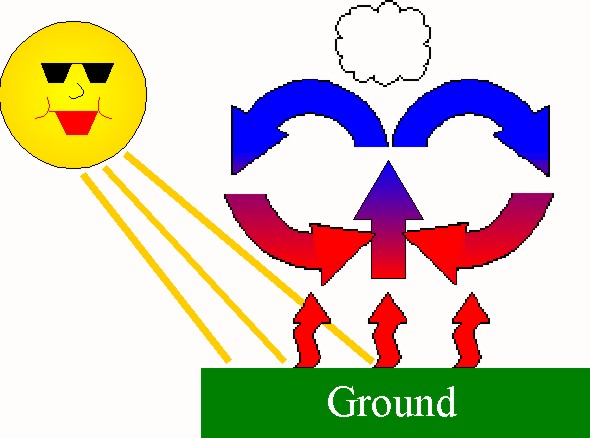
cartoon

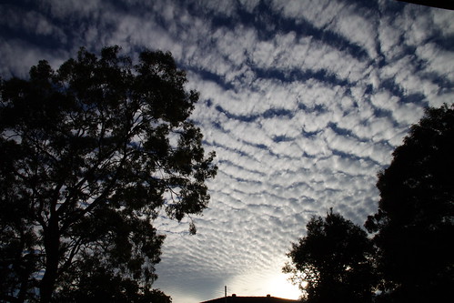
clouds

sketch
Bridge of Schneider Böck: Stability - Instability
And there he is on the bridge,
Cracks! The bridge is falling
apart;

Bild
Linear stability analysis
Consider the continuous dynamical system described by \[ \dot x=f(x,\lambda)\quad \] A bifurcation occurs at \[(x_E,\lambda_0)\] if the Jacobian matrix \[ \textrm{d}f/dx (x_E,\lambda_0)\] has an Eigenvalue with zero real part.
Example: transcritical bifurcation
a fixed point interchanges its stability with another fixed point as the control parameter is varied. Bifurcation at \(r=0\).
\[ \frac{dx}{dt}=rx (1-x) \, \]
The two fixed points are 0 and 1. When r is negative, the fixed point at 0 is stable and 1 is unstable. But for \(r>0\), 0 is unstable and 1 is stable.
Saddle-node bifurcation: two fixed points collide
The normal form: \[ \frac{dx}{dt}=r+x^2 \]
\[ r<0: \mbox{ a stable equilibrium point at } -\sqrt{-r} \mbox{ and an unstable one at } \sqrt{-r} \qquad \qquad \]
\(r=0\): exactly one equilibrium point, saddle-node fixed point.
\(r>0\): no equilibrium points. Saddle-node bifurcations may be associated with hysteresis loops.

Saddle-node bifurcation: two fixed points collide
1) Calculate the equilibrium points:
\[ f(x) = r + x^2 = 0 \]
\[ x_{E1,E2} = \pm \sqrt{-r} \mbox{ for } r \le 0 \]
2) Linear stability conditions for the equilibrium points
\[ f'(x) = 2x \]
\[ f'(x_{E1}) = 2\sqrt{-r} > 0 \quad \mbox{unstable} \]
\[ f'(x_{E2}) = -2\sqrt{-r} < 0 \quad \mbox{stable} \]
For r=0: equilibrium point \(x_E=0\) which is indifferent (not stable/unstable).
Saddle-node bifurcation: two fixed points collide
3) Potential or Lyapunov Method
\[ \frac{dx}{dt}=b+x^2 = - \frac{d}{dx} \left( - b x - \frac{x^3}{3} \right) = - \frac{d}{dx} V (x) \]

Global analysis including basins of attraction for \(x_{E2}: (-\infty,3)\)
dev.new(width=5, height=4, unit=“cm”) \[ x_{E1} = 2\sqrt{9} = 6 \quad \mbox{unstable} \]
\[ x_{E1} = -2\sqrt{9} = -6 \quad \mbox{stable} \]
4) Graphical method: slope at equilibrium points
\[ \frac{dx}{dt}=b+x^2 \]

Bild
filled points: positive slope => unstable
open points: negative slope => stable
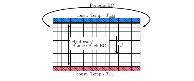
Convection in the Rayleigh-Benard system

Bild
Rayleigh (1916) temperature difference between the upper- and lower-surfaces \[ T(x, y, z=H) = \, T_0 \] \[ T(x, y, z=0) \, = \, T_0 + \Delta T \]
Furthermore \[ \rho = \rho_0 = const. \] except in the buoyancy term, where:
\[ \varrho = \varrho_0 (1 - \alpha(T-T_0)) \mbox{ with } \alpha > 0 \quad . \]
common feature of geophysical flows
No Convection Equilibrium: Diffusion
Bild
Diffusion: Temperature varies linearly with depth:
\[ T_{eq} = T_0 + \left(1 - \frac{z}{H}\right) \Delta T \]
No movement of particles:
\[ u = w= 0 \]
When this solution becomes unstable, convection should develop.
No Convection Equilibrium: Diffusion
Rayleigh-Bénard convection and bifurcation
Experiments:
trailer
Cellules de Bénard (1min),
Rayleigh–Bénard
convection made with mix of cooking oil and small aluminium
particles (5 min),
Was haben
Benard-Zellen mit Kochen zu tun? (3 min, German)
Simulations:
Rayleigh Benard
Thermal Convection with LBM (5 min),
Rayleigh Benard
Thermal Convection 3D Simulation (2 min)
Sketch,
Clouds,
Cartoon
Bifurcations
Bifurcation
youtube (20 min)
Bifurcation Khan
academy (13 min) Reading
Bifurcation theory
Vorticity in the Rayleigh-Benard system
\[ D_t u = - \frac{1}{\rho_0} \partial_x p + \nu \nabla^2 u \label{eqref:einse} \qquad \qquad \qquad \qquad \qquad \qquad (1) \]
\[ D_t w = - \frac{1}{\rho_0} \partial_z p + \nu \nabla^2 w + g (1- \alpha (T-T_0)) \qquad \qquad (2)\]
\[ \partial_x u + \partial_z w = 0 \qquad \qquad \qquad \qquad \qquad \qquad \qquad (3) \]
\[ D_t T = \kappa \nabla^2 T \qquad \qquad \qquad \qquad \qquad \qquad \qquad (4) \]
Introduce vorticity to have (1,2,3) in one equation:
\[ D_t \left( \nabla^2 \Psi\right) = \nu \nabla^4 \Psi - g \alpha \frac{\partial \Theta}{\partial x} \]
Temperature in the Rayleigh-Benard system
\[ T_{eq} = T_0 + \left(1 - \frac{z}{H}\right) \Delta T \]
\[ \mbox{with } \quad T = T_{eq} + \Theta \quad , \quad \mbox{where } \quad \Theta \quad \mbox{is the anomaly} \]
In vorticity equation:
\[ \frac{\partial }{\partial x} g (1- \alpha (T_{eq} + \Theta -T_0)) = - g \alpha \frac{\partial }{\partial x} \Theta \]
Temperature equation:
\[ D_t T = D_t T_{eq} + D_t \Theta = w \cdot \frac{- \Delta T}{H} + D_t \Theta = - \frac{\Delta T}{H} \frac{\partial \Psi}{\partial x} + D_t \Theta \]
\[ D_t \Theta \quad = \frac{\Delta T}{H} \frac{\partial \Psi}{\partial x} + \kappa \nabla^2 \Theta \quad \]
Non-dimensional Rayleigh-Benard system
\[ \frac{1}{T} \frac{1}{L^2} \frac{L^2}{T} D_t \left( \nabla_d^2 \Psi_d\right) = \nu \frac{1}{L^4} \frac{L^2}{T} \nabla_d^4 \Psi_d - g \alpha \frac{ \Delta T}{L} \frac{\partial \Theta_d}{\partial x_d} \]
\[ \frac{\Delta T}{T} D_t \Theta_d \quad = \frac{\Delta T}{H} \frac{L^2}{ T L} \frac{\partial \Psi_d}{\partial x_d} + \kappa \frac{\Delta T}{L^2} \nabla_d^2 \Theta_d \quad \]
This yields (remember \(L=H\)) \[ D_t \left( \nabla_d^2 \Psi_d\right) = \nu \frac{T}{H^2} \nabla_d^4 \Psi_d - g \alpha \frac{T^2 \Delta T}{H} \frac{\partial \Theta_d}{\partial x_d} \] \[ D_t \Theta_d \quad = \frac{\partial \Psi_d}{\partial x_d} + \kappa \frac{T}{H^2} \nabla_d^2 \Theta_d \quad \]
\[ \mbox{Inserting} \quad T= H^2/\kappa \] \[ \mbox{Rayleigh number} \quad R_a = \frac{g \alpha H^3 \Delta T}{\nu \kappa}\] \[ \mbox{Prandtl number} \quad \sigma = \frac{ \nu}{ \kappa} \]
\[ D_t \left( \nabla_d^2 \Psi_d\right) = \frac{ \nu}{ \kappa} \nabla_d^4 \Psi_d - g \alpha \frac{H^3 \Delta T}{\kappa^2} \frac{\partial \Theta_d}{\partial x_d} \label{eqref:psieqnn3} \] \[ D_t \Theta_d \quad = \frac{\partial \Psi_d}{\partial x_d} + \nabla_d^2 \Theta_d \quad . \] Finally, inserting the
\[ D_t \left( \nabla_d^2 \Psi_d\right) = \sigma \nabla_d^4 \Psi_d - R_a \sigma \frac{\partial \Theta_d}{\partial x_d} \]
\[ D_t \Theta_d \quad = \frac{\partial \Psi_d}{\partial x_d} + \nabla_d^2 \Theta_d \quad \]
Galerkin approximation: Get a low-order model
Bild
\[ \mbox{ Saltzman (1962): Expand } \Psi, \Theta \mbox{ in double Fourier series in x and z: } \]
\[ \Psi (x,z,t) \, = \, \sum_{k=1}^\infty \sum_{l=1}^\infty \Psi_{k,l} (t) \, \, \sin \left(\frac{k \pi a}{H} x \right) \, \times \, \sin \left(\frac{ l \pi}{H} z \right) \] \[ \Theta (x,z,t) \, = \, \sum_{k=1}^\infty \sum_{l=1}^\infty \Theta_{k,l} (t) \cos \left(\frac{k \pi a}{H} x \right) \, \times \, \sin \left( \frac{l \pi}{H} z \right) \]
Approximation: Just 3 Modes X(t), Y(t), Z(t)
\[ \frac{a}{1+a^2} \, \kappa \, \Psi = X \sqrt{2} \sin\left(\frac{\pi a}{H} x \right) \sin\left(\frac{\pi}{H} z \right) \]
\[ \pi \frac{R_a}{R_c} \frac{1}{\Delta T} \, \Theta = Y \sqrt{2} \cos\left(\frac{\pi a}{H} x\right) \sin\left(\frac{\pi}{H} z \right) - Z \sin\left(2 \frac{\pi}{H} z \right) \]
Rayleigh number Ra: Buoyancy & Viscosity
\[ \mbox{Motion develops if } \quad R_a = \frac{g \alpha H^3 \Delta T}{\nu \kappa} \quad \mbox{exceeds } \quad R_c = \pi^4 \frac{(1+a^2)^3}{a^2} \]657.51$ occurs when \(a^2 = 1/2\). }$$
\[\mbox{When } R_a < R_c,\mbox{ heat transfer is due to conduction} \]
\[\mbox{When } R_a > R_c, \mbox{ heat transfer is due to convection.} \]
Bild
Lorenz system
Bifurcation at \[ r = R_a/R_c = 1\]
Geometry constant \[b = 4(1+a^2)^{-1}\]
Famous low-order model:
\[ \dot X = -\sigma X + \sigma Y \]
\[ \dot Y = r X - Y - X Z \]
\[ \dot Z = -b Z + X Y \]
\[\mbox{dimensionless time } \quad t_d = \pi^2 H^{-2} (1+a^2) \kappa t,\]
\[ \mbox{ Prandtl number } \quad \sigma = \nu \kappa^{-1}, \]
Lorenz system r=24
left: 52%
r=24
s=10
b=8/3
dt=0.01
x=0.1
y=0.1
z=0.1
vx<-c(0)
vy<-c(0)
vz<-c(0)
for(i in 1:10000){
x1=x+s*(y-x)*dt
y1=y+(r*x-y-x*z)*dt
z1=z+(x*y-b*z)*dt
vx[i]=x1
vy[i]=y1
vz[i]=z1
x=x1
y=y1
z=z1}
plot(vx,vy,type="l",xlab="x",ylab="y")
plot(vy,vz,type="l",xlab="y",ylab="z")

Lorenz system r=0.9
r=0.9
s=10
b=8/3
dt=0.01
x=1.1
y=0.1
z=11.1
vx<-c(0)
vy<-c(0)
vz<-c(0)
for(i in 1:100){
x1=x+s*(y-x)*dt
y1=y+(r*x-y-x*z)*dt
z1=z+(x*y-b*z)*dt
vx[i]=x1
vy[i]=y1
vz[i]=z1
x=x1
y=y1
z=z1}
plot(vx,type="l",xlab="time",ylab="x")
plot(vy,type="l",xlab="time",ylab="y")

Lorenz system r=3.5
r=3.5
s=10
b=8/3
dt=0.01
x=1.1
y=0.1
z=11.1
vx<-c(0)
vy<-c(0)
vz<-c(0)
for(i in 1:1000){
x1=x+s*(y-x)*dt
y1=y+(r*x-y-x*z)*dt
z1=z+(x*y-b*z)*dt
vx[i]=x1
vy[i]=y1
vz[i]=z1
x=x1
y=y1
z=z1}
plot(vx,type="l",xlab="time",ylab="x")
plot(vy,type="l",xlab="time",ylab="y")

Potential vorticity is conserved
\[ \frac{D}{Dt}\left(\zeta+f\right) + \left(\zeta + f\right)\left(\frac{\partial u}{\partial x}+\frac{\partial v}{\partial y}\right)=0 \quad \]
Ocean/Atmosphere with depth h(x,y)
\[ \frac{D}{Dt}\left( \frac{\zeta+f}{h}\right) = 0 \quad \]
Couples depth, vorticity, latitude
– Changes in the depth results in change in \(\zeta\).
– Changes in latitude require a corresponding change in \(\zeta\).

Cape
Dietrich et al. (1980)

Cape
Steward, Oceanography
Angular Momentum and Hadley Cell


Hadely Cell
Tropical air rises to tropopause & moves poleward
Deflected eastward by the Coriolis force
Subtropical jet: forms at poleward limit of Hadley Cell
It tends to conserve angular momentum, friction small
equatorward moving air: westward component
Rotation and Hadley Cell

What drives the ocean currents?
Friction: transfer of momentum from atmosphere to oceanic Ekman layer
Vorticity dynamics for the ocean and include the wind stress term
\[ D_t u - f v = - \frac{1}{\rho} \frac{\partial p}{\partial x} + \frac{1}{\rho} \partial_z \tau_{xz} \] \[ D_t v + f u = - \frac{1}{\rho} \frac{\partial p}{\partial y} + \frac{1}{\rho} \partial_z \tau_{yz} \]
\[ \frac{D}{Dt} \left( {\zeta+f}\right) - \frac{\left(\zeta+f \right)}{h} \frac{D}{Dt} h \, = \, \frac{1}{\rho} \underbrace{\left( \frac{\partial}{\partial x} \, \partial_z \tau_{yz} - \frac{\partial}{\partial y}\, \partial_z \tau_{xz} \right)}_{curl \, \partial_z \tau} \quad . \]
\[ \frac{D}{Dt} \left( \frac{\zeta+f}{h}\right) = \frac{1}{\rho \, h} \, \mbox{curl} \, \partial_z \tau \, \]
Sverdrup transport

Sverdrup
applied globally using the wind stress from Hellerman and Rosenstein (1983). Contour interval is \(10\) Sverdrups (Tomczak and Godfrey, 1994).
\[ \beta v = \frac{1}{\rho } \, \mbox{curl} \, \partial_z \tau \, \]
\[ \int_{-H}^0 dz \, \beta v = \frac{1}{\rho } \, \int_{-H}^0 dz \, \mbox{curl} \, \partial_z \tau \, = \frac{1}{\rho } \, \mbox{curl} \, \tau \, \]
\[ V = \frac{1}{\rho \beta} \, \left( \frac{\partial \tau_{yz} }{\partial x} \, - \frac{\partial \tau_{xz}}{\partial y}\, \right) = \frac{1}{\rho \beta} \, \, \operatorname{curl} \, \tau \]
Ekman Pumping: vertical velocity at the bottom of the Ekman layer E
\(w_E\) as the Ekman vertical velocity the bottom of the Ekman layer \[ w_E = - \int_{-E}^0 \frac{\partial w}{\partial z} dz = \frac{\partial}{\partial x} U_E + \frac{\partial}{\partial y} V_E \]
\(\operatorname{curl} \mathbf{\tau}\) produces a divergence of the Ekman transports leading to \(w_E\) at the bottom E
\[ w_E = \, \frac{\partial }{\partial x} \left( \frac{ \tau_{y}}{\rho \;f }\, \right) - \frac{\partial }{\partial y}\, \left( \frac{ \tau_{x}}{\rho \;f }\, \right) =\operatorname{curl}\left(\frac{\mathbf{\tau}}{\rho\;f}\right) \simeq \frac{1}{\rho\;f} \, \operatorname{curl} \mathbf{\tau} \]
The order of magnitude of the Ekman vertical velocity:
typical wind stress variation of \(0.2 N m^{-2}\) per 2000 km in y-direction:
\[ w_E \simeq - \frac{ \Delta \tau_{x}}{\rho \;f_0 \Delta y}\, \simeq \frac{1 }{10^3 kg m^{-3}} \frac{0.2 N m^{-2} }{10^{-4} s^{-1}\, \, 2 \cdot 10^6 m} \simeq 32 \, \, \frac{m}{yr} \]
Ekman Pumping & Sverdrup Transport

Ekman
The center of a subtropical gyre is a high pressure zone: clockwise on the Northern Hemisphere
Ekman surface currents towards the center of the gyre
The Ekman vertical velocity balanced by \[ w_E=w_g \] vertical geostrophic current in the interior
geostrophic flow towards the equator
returned flow towards the pole in western boundary currents
North Atlantic Current & Gulfstream

Gulf Stream & North Atlantic Current

Part of deep ocean
brings warm water northward where it cools.
returns southward as a cold, deep, western-boundary current.
Gulf Stream carries 40 Sv of 18°C water northward.
Of this, 15 Sv return southward in the deep western boundary current at a temperature of 2°C.
How much heat is transported northward ?
Calculation:
\[ \underbrace{ c_p}_{4.2 \cdot 10^3 Ws/(m^3 kg)} \, \cdot \, \underbrace{ \rho }_{10^3 kg/m^3 } \, \cdot \, \underbrace{\Phi}_{15 \cdot 10^6 m^3/s} \, \cdot \, \underbrace{\Delta T}_{(18-2) K } = 1 \cdot 10^{15} W \]
The flow carried by the conveyor belt loses 1 Petawatts (PW), close to estimates of Rintoul and Wunsch (1991)
The deep bottom water from the North Atlantic is mixed upward in other regions and ocean, and it makes its way back to the Gulf Stream and the North Atlantic. Thus most of the water that sinks in the North Atlantic must be replaced by water from the far South Atlantic and Pacific Ocean.
Conveyor Belt

Conveyor
Conveyor Belt

Conveyor
Conveyor belt circulation
The the conveyor is driven by deepwater formation in the northern North Atlantic.
The conveyor belt metaphor necessarily simplifies the ocean system, it is of course not a full description of the deep ocean circulation.
Broecker’s concept provides a successful approach for global ocean circulation, although several features can be wrong like the missing Antarctic bottom water, the upwelling areas etc..
metaphor inspired new ideas of halting or reversing the ocean circulation and put it into a global climate context.
interpretation of Greenland ice core records indicating different climate states with different ocean modes of operation (like on and off states of a mechanical maschine).
Thermohaline ocean circulation

Overturning
Modelled meridional overturning streamfunction in Sv 10^6 = m^3 /s in the Atlantic Ocean. Grey areas represent zonally integrated smoothed bathymetry
Meteor

Meteor
Meteor Expedition, the first accurate hydrographic survey of the Atlantic from Wuest (1935).
Meteor

Temp & salinity
Meteor Expedition, the first accurate hydrographic survey of the Atlantic from Wuest (1935).
Estimates of overturning ?
It is observed that water sinks in to the deep ocean in polar regions of the Atlantic basin at a rate of 15 Sv. (Atlantic basin: 80,000,000 km^2 area * 4 km depth.)
– How long would it take to ‘fill up’ the Atlantic basin?
– Supposing that the local sinking is balanced by large-scale upwelling, estimate the strength of this upwelling.
Hint: Upwelling = area * w
– Compare this number with that of the Ekman pumping!
Estimates of overturning
Timescale T to ‘fill up’ the Atlantic basin:
\[ T = \frac{ 80 \cdot 10^{12} \, m^2 \cdot 4000 \, m}{15 \cdot 10^6 \, m^3 s^{-1}} = 2.13 \cdot 10^{10} s = 676 \;years\]
Overturning is balanced by large-scale upwelling:
\[ area \cdot w = 15 \cdot 10^6 \, m^3 s^{-1}\]
\[ w = 0.1875 \cdot 10^{-6} m\;s^{-1} = 5.9 \cdot 10^{-15} m \; y^{-1}. \]
Ekman pumping \[ w_E \simeq 32 \, \, m \; y^{-1}. \]
Vorticity dynamics of meridional overturning (y,z)
\[ \frac{\partial}{\partial t} v \quad = \quad - \frac{1}{\rho_0} \frac{\partial p}{\partial y} \quad - \quad f u \quad - \quad \kappa v \]
\[ \frac{\partial}{\partial t} w \quad = \quad - \frac{1}{\rho_0} \frac{\partial p}{\partial z} \quad - \quad \frac{g}{\rho_0} (\rho -\rho_0) \quad - \quad \kappa w \] \(\kappa\) as parameter for Rayleigh friction.
Using the continuity equation
\[
0 \quad = \quad \frac{\partial v}{\partial y} \quad +
\quad \frac{\partial w}{\partial z}
\]
\[ \mbox{ one can introduce a streamfunction } \Phi (y,z): v= \partial_z \Phi; w = - \partial_y \Phi \]
The associated vorticity equation in the (y,z)-plane is therefore
\[ \frac{\partial}{\partial t} \nabla^2 \Phi \, = \, - f \frac{\partial u}{\partial z} \quad + \quad \frac{g}{\rho_0} \frac{\partial \rho}{\partial y} \quad - \quad \kappa \nabla^2 \Phi \]
Galerkin approximation
\[ {\frac{\partial}{\partial t} \nabla^2 \Phi} \, = \, \underbrace{- f \frac{\partial u}{\partial z}}_{2.} \quad + \quad { \frac{g}{\rho_0} \frac{\partial \rho}{\partial y}} \quad - \quad \underbrace{ \kappa \nabla^2 \Phi }_{4.} \]
Term 2. is absorbed into the viscous term (4.)
\[ \Phi (y,z,t) \, = \, \sum_{k=1}^\infty \sum_{l=1}^\infty \Phi_{max}^{k,l} (t) \, \, \sin (\pi k y/L) \, \times \, \sin (\pi l z/H) \] yielding a first order differential equation in time for \(\Phi_{max}^{k,l} (t)\).
Simple ansatz satisfying that the normal velocity at the boundary vanishes \[ \Phi (y,z,t) \, = \, \Phi_{max} (t) \, \, \sin \left(\frac{\pi y}{L}\right) \, \times \, \sin \left(\frac{\pi z}{H}\right) \]
L and H dentote the meridional and depth extend: y from 0 to L, z from 0 to H
The remaining terms and integration
\[ \underbrace{\int_0^L dy \int_0^H dz \quad \frac{\partial}{\partial t} \nabla^2 \Phi}_{1.} \, = \, \underbrace{ \int_0^L dy \int_0^H dz \quad \frac{g}{\rho_0} \frac{\partial \rho}{\partial y}}_{2.} \quad - \underbrace{ \int_0^L dy \int_0^H dz \quad \kappa \nabla^2 \Phi }_{3.} \]
- \[ \frac{d}{dt} \Phi_{max} \left(\frac{\pi^2}{L^2} + \frac{\pi^2}{H^2}\right) \int\limits_0^L dy \sin \left(\frac{\pi y}{L}\right) \int\limits_0^H dz \sin \left(\frac{\pi z}{H}\right) = 4 LH \left(\frac{1}{L^2} + \frac{1}{H^2}\right) \frac{d}{dt} \Phi_{max} \]
The remaining terms and integration
\[ \underbrace{\int_0^L dy \int_0^H dz \quad \frac{\partial}{\partial t} \nabla^2 \Phi}_{1.} \, = \, \underbrace{ \int_0^L dy \int_0^H dz \quad \frac{g}{\rho_0} \frac{\partial \rho}{\partial y}}_{2.} \quad - \underbrace{ \int_0^L dy \int_0^H dz \quad \kappa \nabla^2 \Phi }_{3.} \]
\[ \frac{d}{dt} \Phi_{max} \left(\frac{\pi^2}{L^2} + \frac{\pi^2}{H^2}\right) \int\limits_0^L dy \sin \left(\frac{\pi y}{L}\right) \int\limits_0^H dz \sin \left(\frac{\pi z}{H}\right) = 4 LH \left(\frac{1}{L^2} + \frac{1}{H^2}\right) \frac{d}{dt} \Phi_{max} \]
\[ \int\limits_0^L dy \int\limits_0^H dz \frac{g}{\rho_0} \frac{\partial \rho}{\partial y} = \frac{g}{\rho_0} \, H \, (\rho_{north} - \rho_{south}) \quad \mbox{ with } \rho_{north} = \rho (y=L) , \rho_{south} = \rho (y=0) \]
=======================================================
\[ \underbrace{\int_0^L dy \int_0^H dz \quad \frac{\partial}{\partial t} \nabla^2 \Phi}_{1.} \, = \, \underbrace{ \int_0^L dy \int_0^H dz \quad \frac{g}{\rho_0} \frac{\partial \rho}{\partial y}}_{2.} \quad - \underbrace{ \int_0^L dy \int_0^H dz \quad \kappa \nabla^2 \Phi }_{3.} \]
\[ \frac{d}{dt} \Phi_{max} \left(\frac{\pi^2}{L^2} + \frac{\pi^2}{H^2}\right) \int\limits_0^L dy \sin \left(\frac{\pi y}{L}\right) \int\limits_0^H dz \sin \left(\frac{\pi z}{H}\right) = 4 LH \left(\frac{1}{L^2} + \frac{1}{H^2}\right) \frac{d}{dt} \Phi_{max} \]
\[ \int\limits_0^L dy \int\limits_0^H dz \frac{g}{\rho_0} \frac{\partial \rho}{\partial y} = \frac{g}{\rho_0} \, H \, (\rho_{north} - \rho_{south}) \quad \mbox{ with } \rho_{north} = \rho (y=L) , \rho_{south} = \rho (y=0) \]
\[ \kappa \Phi_{max} \left(\frac{\pi^2}{L^2} + \frac{\pi^2}{H^2}\right) \int\limits_0^L dy \sin \left(\frac{\pi y}{L}\right) \int\limits_0^H dz \sin \left(\frac{\pi z}{H}\right) = \kappa \, 4 LH \left(\frac{1}{L^2} + \frac{1}{H^2}\right) \Phi_{max} \]
Amplitude of overturning
\[ \frac{d}{dt} \Phi_{max} \, = \, \frac{a}{\rho_0} (\rho_{north} - \rho_{south}) \, \, - \, \, \kappa \Phi_{max} \]
with \[ a = g L H^2/4(L^2 + H^2) \, \]
This shows that the overturning circulation depends on the density differences on the right and left boxes.
It is simplified to a diagnostic relation
\[ \Phi_{max} = \frac{a}{\rho_0 \, \kappa} \, \, (\rho_{north} - \rho_{south}) \quad \]
because the adjustment of \(\Phi_{max}\) is quasi-instantaneous due to adjustment processes, e.g. Kelvin waves.
=======================================================

THC
Schematic picture of the hemispheric two box model (a) and of the interhemispheric box model
=======================================================

THC
The Atlantic surface density is mainly related to temperature differences.
But the pole-to-pole differences are caused by salinity differences. }