Dynamics II: lecture 5
Gerrit Lohmann date: May 17, 2021
Organization of
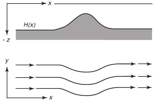
Potential vorticity is conserved
\[ \frac{D}{Dt}\left(\zeta+f\right) + \left(\zeta + f\right)\left(\frac{\partial u}{\partial x}+\frac{\partial v}{\partial y}\right)=0 \quad \]
Couples depth, vorticity, latitude
– Changes in the depth results in change in \( \zeta \).
– Changes in latitude require a corresponding change in \( \zeta \).
Dietrich et al. (1980)
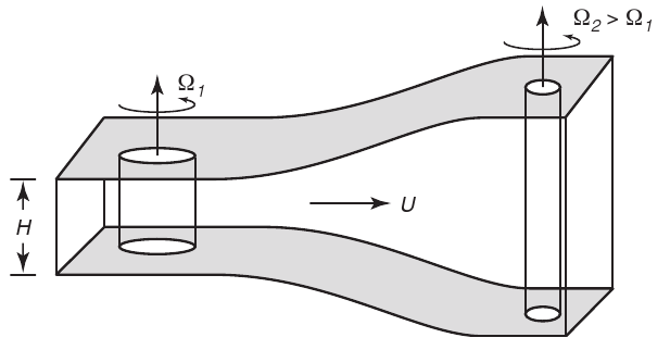
Ocean with depth h(x,y)
\[ \frac{D}{Dt}\left( \frac{\zeta+f}{h}\right) = 0 \quad \]
Steward, Oceanography
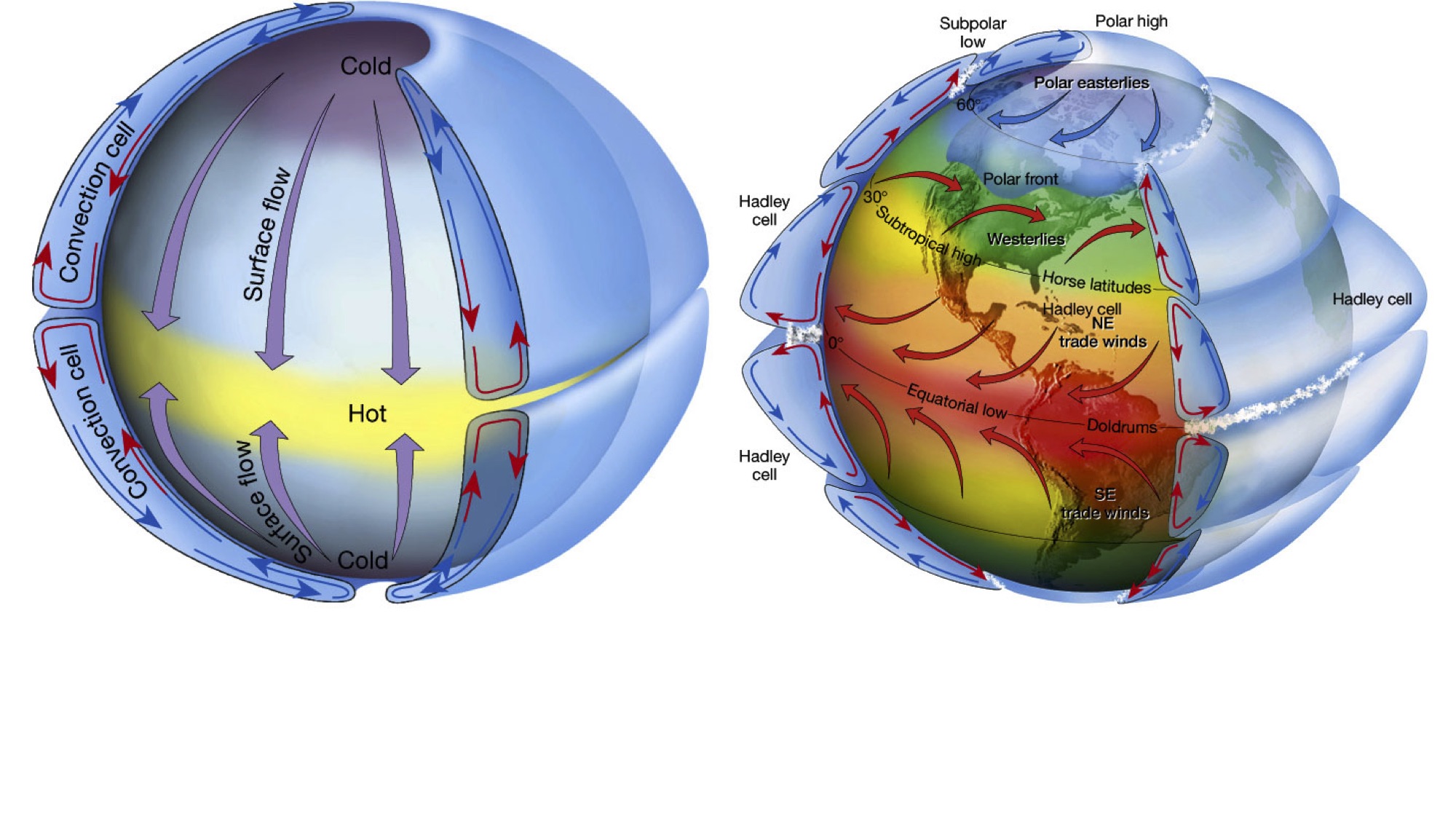
Angular Momentum and Hadley Cell
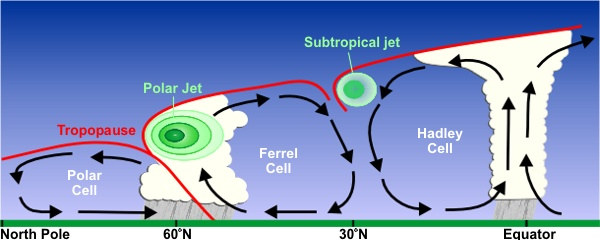
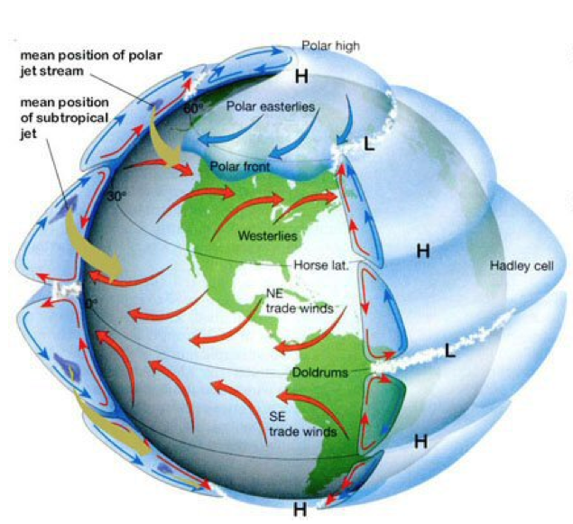
Rotation and Hadley Cell
What drives the ocean currents?
Sverdrup transport
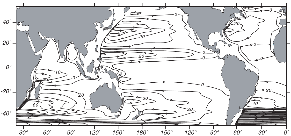
applied globally using the wind stress from Hellerman and Rosenstein (1983). Contour interval is \( 10 \) Sverdrups (Tomczak and Godfrey, 1994).
\[ V = \frac{1}{\rho \beta} \, \left( \frac{\partial \tau_{yz} }{\partial x} \, - \frac{\partial \tau_{xz}}{\partial y}\, \right) = \frac{1}{\rho \beta} \, \, \operatorname{curl} \, \tau \]
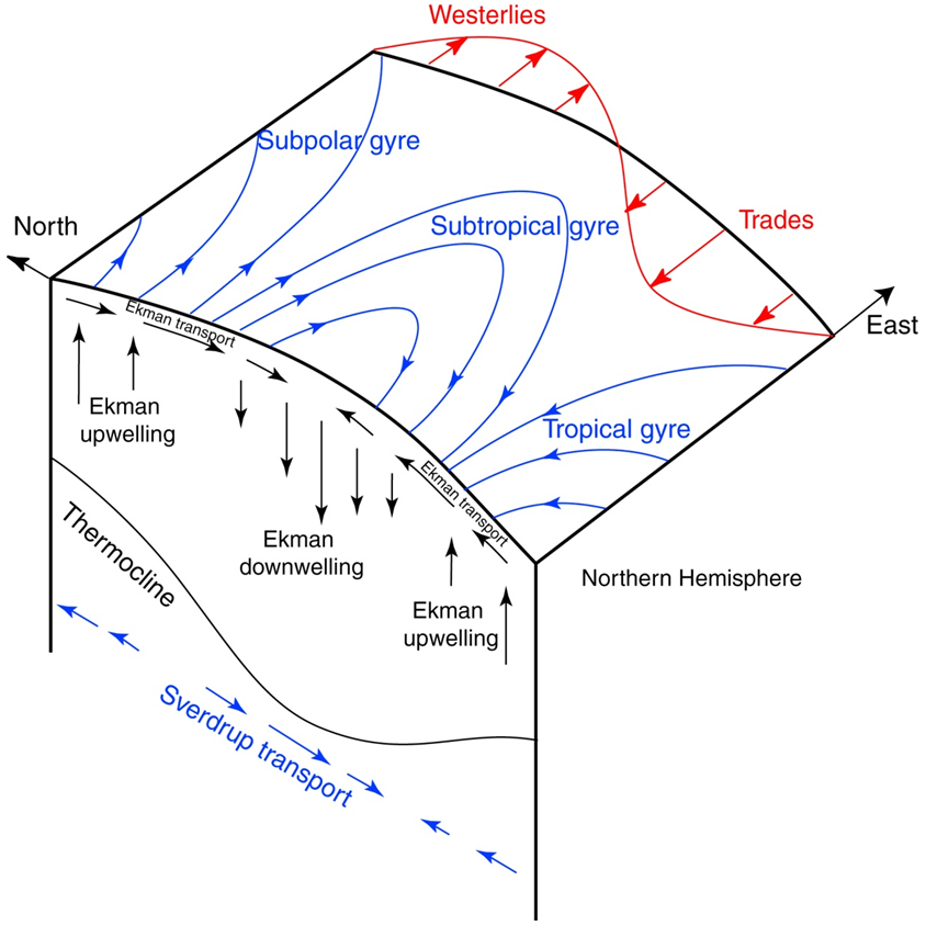
Ekman Pumping: vertical velocity at the bottom
Ekman Pumping & Sverdrup Transport
North Atlantic Current & Gulfstream
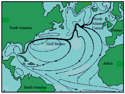
brings warm water northward where it cools.
returns southward as a cold, deep, western-boundary current.
North Atlantic Current & Gulfstream
brings warm water northward where it cools.
returns southward as a cold, deep, western-boundary current.
North Atlantic Current & Gulfstream
brings warm water northward where it cools.
returns southward as a cold, deep, western-boundary current.
Conveyor Belt
Conveyor Belt

Conveyor belt circulation
Thermohaline ocean circulation
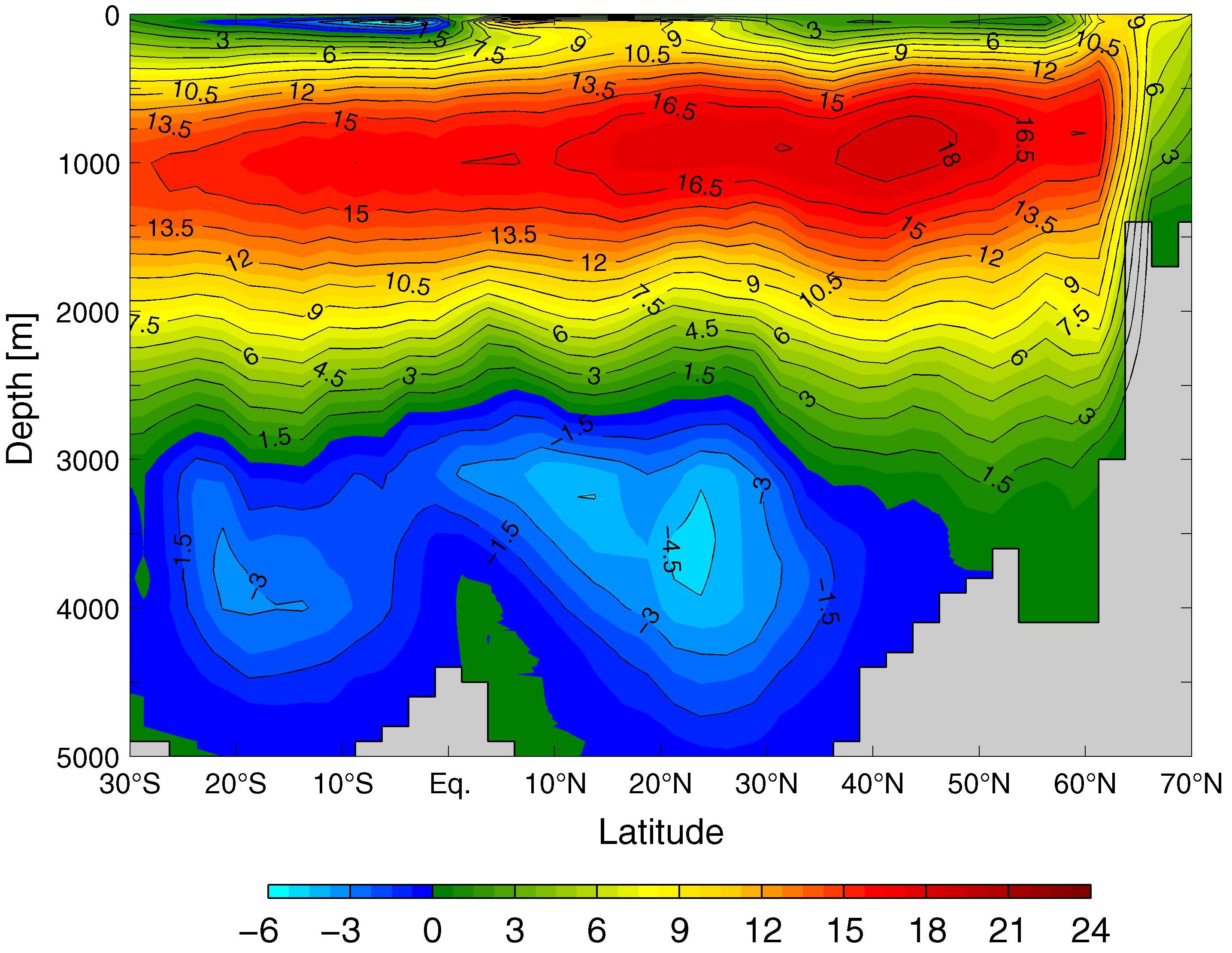 Modelled meridional overturning streamfunction in Sv 106 = m3 /s in the Atlantic Ocean. Grey areas represent zonally integrated smoothed bathymetry
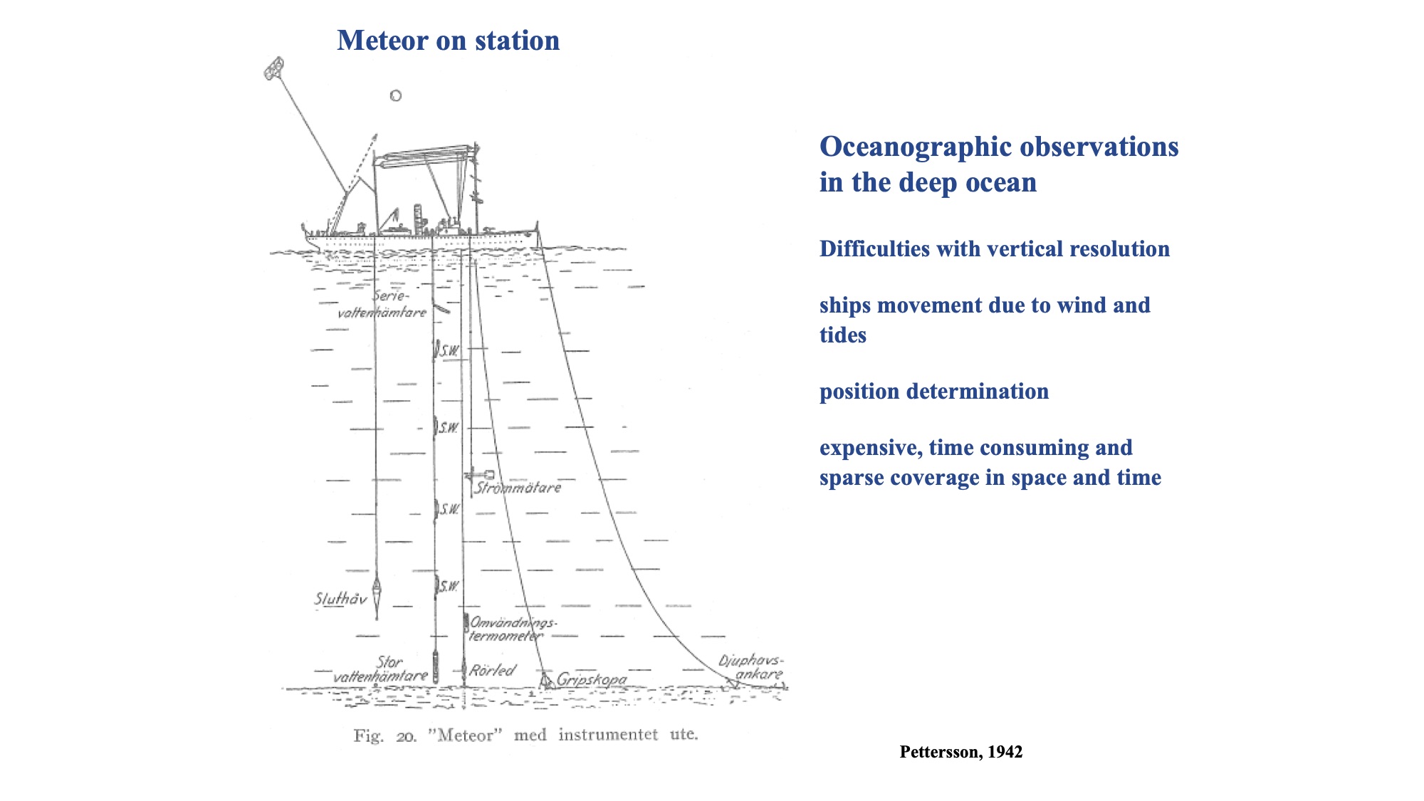
Meteor
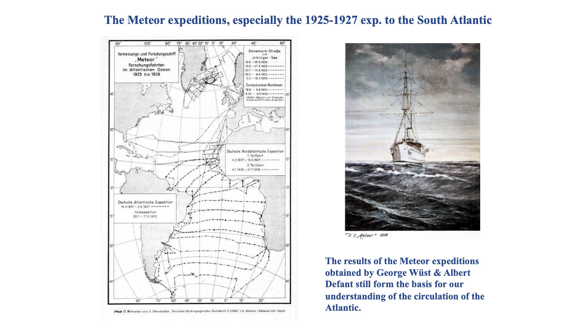
Meteor Expedition, the first accurate hydrographic survey of the Atlantic from Wuest (1935).
Meteor
Meteor Expedition, the first accurate hydrographic survey of the Atlantic from Wuest (1935).
Meteor
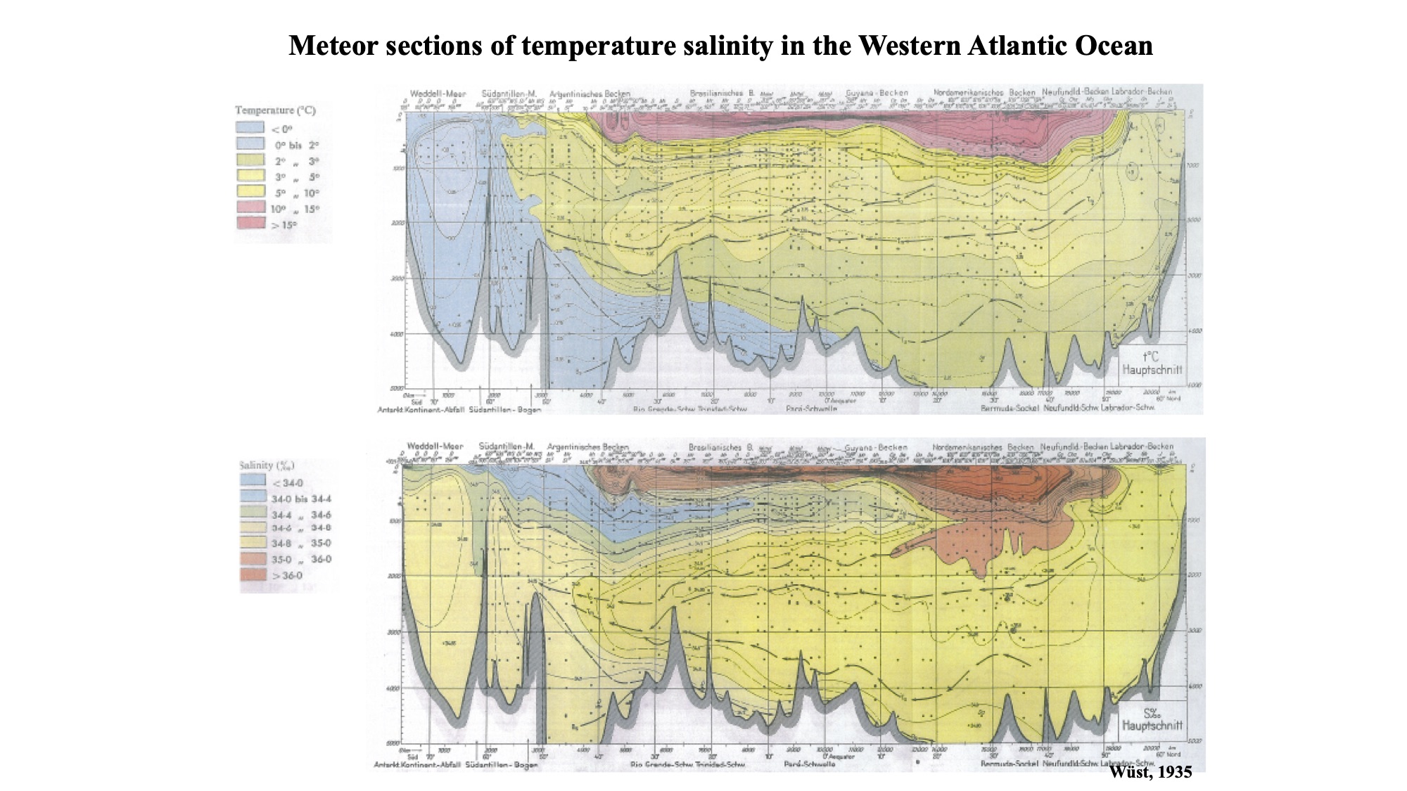
Lower panel: Salinity and dissolved oxygen on the Hauptschnitt along the western side of the Atlantic.
Estimates of overturning ?
Estimates of overturning
Vorticity dynamics of meridional overturning (y,z)
Vorticity dynamics of meridional overturning (y,z)
Galerkin approximation
The remaining terms and integration
The remaining terms and integration
Amplitude of overturning
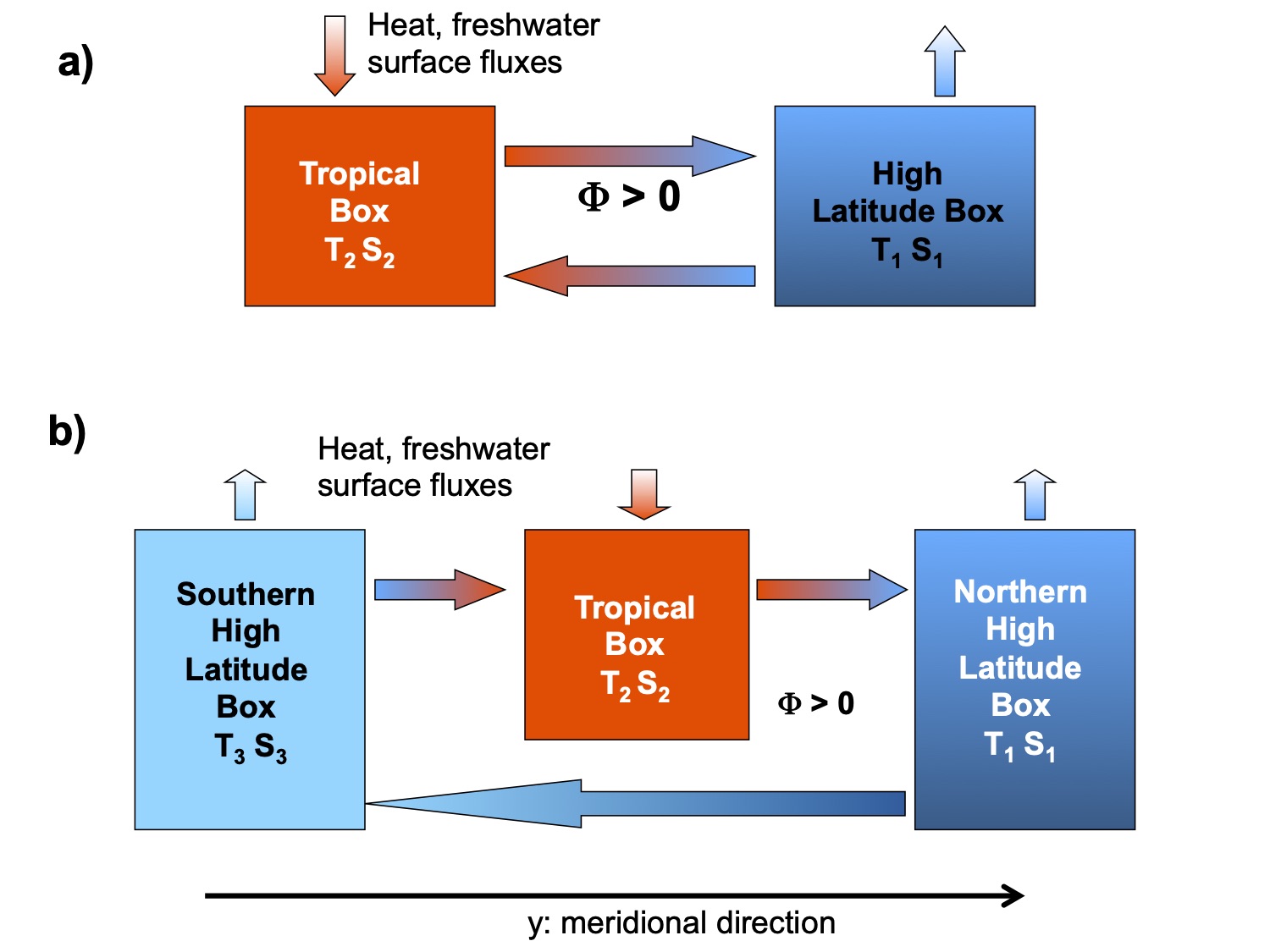
Schematic picture of the hemispheric two box model (a) and of the interhemispheric box model
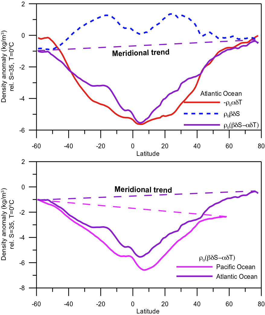
a) The Atlantic surface density is mainly related to temperature differences. b) But the pole-to-pole differences are caused by salinity differences. }