Dynamics II
Lecture: May 22, 2023 (Monday), 14:00 Prof. Dr. Gerrit Lohmann
Preparation
Chapter The equations of fluid motion (Marchal and Plumb, 2008)
Video Introduction to Atmospheric Dynamics (47 min)
Basics in Chapter 1 “The Equations of Atmospheric Dynamics” Holton and Hakim (2013)
May be you have already installed R (https://www.r-project.org) and the RStudio (https://www.rstudio.com). you can install the rmarkdown package in R:
# Install from CRAN
install.packages(‘rmarkdown’)
Content for today
May 22, 14:00: Lecture 5 (G. Lohmann)
Content for today: Fluid Dynamics, Non-dimensional parameters, Dynamical similarity, Elimination of the pressure term and vorticity, bifurcations, applications
Basics of Fluid Dynamics
a model describes the state variables, plus fundamental laws and equations of state.
- State variables: Velocity (in each of three directions), pressure, temperature, salinity, density, etc.
- Fundamental laws: Conservation of momentum, conservation of mass, conservation of temperature and salinity
- Equations of state: Relationship of density to temperature, salinity and pressure, etc.
Material laws
The effect of stress represented by \(\nabla p\) and \(\nabla \cdot\mathbb{T}\) terms.
\(\nabla p\) is called the pressure gradient and arises from the isotropic part of the stress tensor.
The anisotropic part of the stress tensor gives rise to \(\nabla \cdot\mathbb{T},\) describing viscous forces.
The stress terms p and \(\mathbb{T}\) are yet unknown: a force model is needed relating the stresses to the fluid motion.
Assumptions on the specific behavior of a fluid are made (based on observations).
The Cauchy stress tensor can be also written in matrix form: \[ \mathbb{T} = \left({\begin{matrix} \mathbf{T}^{(\mathbf{e}_1)} \\ \mathbf{T}^{(\mathbf{e}_2)} \\ \mathbf{T}^{(\mathbf{e}_3)} \\ \end{matrix}}\right) = \left({\begin{matrix} \sigma _{11} & \sigma _{12} & \sigma _{13} \\ \sigma _{21} & \sigma _{22} & \sigma _{23} \\ \sigma _{31} & \sigma _{32} & \sigma _{33} \\ \end{matrix}}\right) \equiv \left({\begin{matrix} \sigma _{xx} & \sigma _{xy} & \sigma _{xz} \\ \sigma _{yx} & \sigma _{yy} & \sigma _{yz} \\ \sigma _{zx} & \sigma _{zy} & \sigma _{zz} \\ \end{matrix}}\right) \equiv \left({\begin{matrix} \sigma _x & \tau _{xy} & \tau _{xz} \\ \tau _{yx} & \sigma _y & \tau _{yz} \\ \tau _{zx} & \tau _{zy} & \sigma _z \\ \end{matrix}}\right) \label{eqn:T} \]
where \(\sigma\) are the normal stresses and \(\tau\) are the shear stresses. From the Newton’s third law (actio est reactio), the stress tensor is symmetrical: \[ \mathbb{T} = \mathbb{T}^T \]
In the Figure the stress vectors \(\mathbf{T}^{(\mathbf{e}_{i})}\) can be decomposed in one normal stress and two shear stress components.
 Components of stress in three dimensions.
Conservation of mass
Regardless of the flow assumptions, a statement of the conservation of mass is generally necessary. This is achieved through the mass continuity equation, given in its most general form as: \[ \frac{\partial \rho}{\partial t} + \nabla \cdot (\rho \mathbf{u}) = 0 \] or, using the substantive derivative: \[ \frac{D\rho}{Dt} + \rho (\nabla \cdot \mathbf{u}) = 0. \]
Exercise advection
The temperature at a point 50 km north of a station is 3\(^\circ\)C cooler than at the station. If the wind is blowing from the northeast at 20m/s and the air is being heated by radiation at a rate of 1\(^\circ\)C/h, what is the local temperature change at the station?
Solution of Temperature Advection
The total change of temperature is given by \[ \frac{d T}{dt} = \frac{\partial T}{\partial t} + {\bf u} \cdot \nabla T = \dot{q} \] \[ \Leftrightarrow \quad \frac{\partial T}{\partial t} = - {\bf u} \cdot \nabla T + \dot{q} \] Here we use the velocity \[ {\bf u} = - 20 \frac{m}{s} \cdot \frac{1}{\sqrt{2}} (1, 1, 0) , \qquad \nabla T = \frac{{3}{^\circ C}}{{50}{km}} (0, -1, 0), \qquad \dot{q} = 1 \frac{^\circ C}{h} \] Then we calculate the temperature change at the station \[ \frac{\partial T}{\partial t} = - {\bf u} \cdot \nabla T + \dot{q} \]
\[ \frac{\partial T}{\partial t} = 20 \frac{m}{s} \, \frac{1}{\sqrt{2}} (1, 1, 0) \cdot (0, -1, 0) \frac{{3}{^\circ C}}{{50}{km}} + 1 \frac{^\circ C}{h} \approx {-2.1} \frac{^\circ C}{h} \]
Elimination of the pressure term
in the 2D-Navier-Stokes equation.
2D: assume \(w = 0\) and no dependence of anything on z
\[ \rho \left(\frac{\partial u}{\partial t} + u \frac{\partial u}{\partial x} + v \frac{\partial u}{\partial y}\right) = -\frac{\partial p}{\partial x} + \mu \left(\frac{\partial^2 u}{\partial x^2} + \frac{\partial^2 u}{\partial y^2}\right) \] \[ \rho \left(\frac{\partial v}{\partial t} + u \frac{\partial v}{\partial x} + v \frac{\partial v}{\partial y}\right) = -\frac{\partial p}{\partial y} + \mu \left(\frac{\partial^2 v}{\partial x^2} + \frac{\partial^2 v}{\partial y^2}\right) \]
Procedure
Differentiating the first with respect to y: \[\partial_y\]
the second with respect to x: \[\partial_x\]
and subtracting the resulting equations will eliminate pressure and any potential force.
Defining the stream function \(\psi\) through \[ u = \frac{\partial \psi}{\partial y} \quad ; \quad v = -\frac{\partial \psi}{\partial x} \]
results in mass continuity being unconditionally satisfied (given the stream function is continuous), and then incompressible Newtonian 2D momentum and mass conservation degrade into one equation:
\[ \frac{\partial}{\partial t}\left(\nabla^2 \psi\right) + \frac{\partial \psi}{\partial y} \frac{\partial}{\partial x}\left(\nabla^2 \psi\right) - \frac{\partial \psi}{\partial x} \frac{\partial}{\partial y}\left(\nabla^2 \psi\right) = \nu \nabla^4 \psi \]
or using the total derivative\[ D_t \left(\nabla^2 \psi\right) = \nu \nabla^4 \psi \] \(\nabla^4\) is the (2D) biharmonic operator and \(\nu\) the kinematic viscosity \(\nu=\frac{\mu}{\rho}.\)
This single equation describes 2D fluid flow, kinematic viscosity as parameter!
The concept will become very important in ocean dynamics. The term \[\zeta=\nabla^2 \psi\]
is called relative vorticity, its dynamics can be described as \[ D_t \zeta = \nu \nabla^2 \zeta \quad \]
Non-dimensional parameters: The Reynolds number
For the case of an incompressible flow in the Navier-Stokes equations, assuming the temperature effects are negligible and external forces are neglected.
conservation of mass \[ \nabla \cdot \mathbf{u} = 0 \] conservation of momentum \[ \partial_t \mathbf{u} + ( \mathbf{u} \cdot \nabla) \mathbf{u} = - \frac{1}{\rho_0} \nabla p + \nu \nabla^2 \mathbf{u} \]
The equations can be made dimensionless by a length-scale L, determined by the geometry of the flow, and by a characteristic velocity U.
For analytical solutions, numerical results, and experimental measurements, it is useful to report the results in a dimensionless system (concept of dynamic similarity).
Goal: replace physical parameters with dimensionless numbers, which completely determine the dynamical behavior
representative values for velocity \((U),\) time \((T),\) distances \((L)\)
Using these values, the values in the dimensionless-system (written with subscript d) can be defined: \[ u =U \cdot u_d \] \[ t = T \cdot t_d \] \[ x = L \cdot x_d \] with \(U = L/T\).
From these scalings, we can also derive \[ \partial_t = \frac{\partial}{\partial t } = \frac{1}{T} \cdot \frac{\partial}{\partial t_d } \] \[ \partial_x = \frac{\partial}{\partial x} = \frac{1}{L} \cdot \frac{\partial}{\partial x_d } \] Note furthermore the units of \([\rho_0] = kg/m^3\), \([p] = kg/(m s^2)\), and \([p]/[\rho_0]= m^2/s^2\). Therefore the pressure gradient term has the scaling \(U^2/L\).
\[ \nabla_d \cdot \mathbf{u_d} = 0 \] and conservation of momentum
…
The dimensionless parameter \[ Re=UL/ \nu \]
is the Reynolds number and the only parameter left!
For large Reynolds numbers, the flow is turbulent.
In most practical flows \(Re\) is rather large \((10^4-10^8),\) large enough for the flow to be turbulent. A large Reynolds number allows the flow to develop steep gradients locally.
In the literature, the term “equations have been made dimensionless”, means that this procedure is applied and the subscripts d are dropped.
Characterising flows by dimensionless numbers
These numbers can be interpreted as follows:
- Re: (stationary inertial forces)/(viscous forces)
- Sr: (non-stationary inertial forces)/(stationary inertial forces)
- Fr: (stationary inertial forces)/(gravity)
- Fo: (heat conductance)/(non-stationary change in enthalpy)
- Pe: (convective heat transport)/(heat conductance)
- Ec: (viscous dissipation)/(convective heat transport)
- Ma: (velocity)/(speed of sound): objects moving faster than 0.8 produce shockwaves
- Pr and Nu are related to specific materials.
Rayleigh-Benard convection (and Rayleigh number)
Experiments:
Rayleigh–Bénard convection: cooking oil and small aluminium particles (5 min),
Rayleigh Benard
Thermal Convection 3D Simulation (2 min)

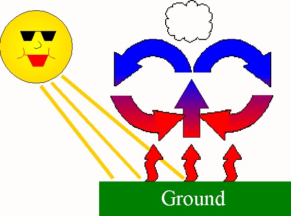
cartoon

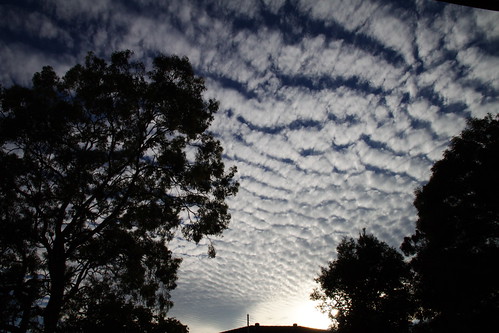
clouds

sketch
Bifurcations
Bifurcation
youtube, Bifurcation Khan
academy, Bifurcation
K
Max and
Moritz, not lazy, sawing secretly a gap in the bridge.
When now
this act is over, you suddenly hear a scream:
“Hey, out! You billy
goat!
Tailor, tailor, bitch, bitch, bitch!”

Bridge of Schneider Böck: Stability - Instability
And there he is on the bridge,
Cracks! The bridge is falling
apart;

Bild
Linear stability analysis
Consider the continuous dynamical system described by \[ \dot x=f(x,\lambda)\quad \] A bifurcation occurs at \[(x_E,\lambda_0)\] if the Jacobian matrix \[ \textrm{d}f/dx (x_E,\lambda_0)\] has an Eigenvalue with zero real part.
Example: transcritical bifurcation
a fixed point interchanges its stability with another fixed point as the control parameter is varied. Bifurcation at \(r=0\).
\[ \frac{dx}{dt}=rx (1-x) \, \]
The two fixed points are 0 and 1. When r is negative, the fixed point at 0 is stable and 1 is unstable. But for \(r>0\), 0 is unstable and 1 is stable.
Stability - Instability: Consumer-producer problem
A typical example could be the consumer-producer problem where the consumption is proportional to the (quantity of) resource.
For example:
\[ \frac{dx}{dt}=rx(1-x)-px \]
where
\[ rx(1-x) \]
is the logistic equation of resource growth:
Rate of reproduction proportional to the population, available resources
\(px\): Consumption, proportional to the resource x.
\[ x_{E 1} = 0, \mbox{ and } x_{E 2 } = 1 - \frac{p}{r} \]
Logistic equation of population growth
Verhulst: describe the self-limiting growth of a biological population with size N:
\[ \frac{dN}{dt}=r N \cdot \left( 1- \frac{N}{K} \right) \]
r growth rate and K carrying capacity.
the early, unimpeded growth rate is modeled by the first term \(r N.\)
“Bottleneck” is modeled by the value of K.
As the population grows, \(-r N^2/K\) becomes large as some members interfere with each other by competing for some critical resource (food, living space). The competition diminishes the combined growth rate, until the value of N ceases to grow (maturity of the population).
\[ N(t) = \frac{K N_0 e^{rt}}{K + N_0 \left( e^{rt} - 1\right)} = \frac{K }{K/N_0 e^{-rt} + 1- e^{-rt} } \quad \rightarrow_{t\to \infty } K \]
In climate, the logistic equation is also important for Lorenz’s forecast error.
Human population: logistic growth model

Bild

Bild
Explosion of human population over the last 10,000
years along with some relevant historical events.
Think about the ways that each of these events might have affected birth and death rates of the human population.
Coronavirus epidemic: logistic growth model
left: 35%

Bild Corona
N is the number of cases,
r infection rate,
p cure rate,
K final epidemic size.
dN/dt linearly decreases with the number of cases.
\[ \frac{dN}{dt}=r N \cdot \left( 1- \frac{N}{K} \right) - p N \]
Questions:
When is the growth rate peak?
How many infections ?
When do we need places in hospitals?
r=2000/150000
left: 50%
r=2000/150000
Bev=85000000
K=1
dt=0.01
N=150000/Bev
vN=c(0); vNp=c(0); vt=c(0)
vN[1]=N; vNp[1]=0; vt[1]=0
for(i in 2:100000){
N1=N+r*N*(1-N/K)*dt
vNp[i]=r*N*(1-N/K)
vN[i]=N1
vt[i]=i*dt
N=N1}
plot(vt,vN,type="l",xlab="time [days]",ylab="N(t)")
plot(vt,vNp*Bev/100,type="l",xlab="time [days]",ylab="dN(t)/dt * 1/100 ")
max(vNp[]*Bev/100)

## [1] 2833.333r=5000/150000
left: 50%
r=5000/150000
Bev=85000000
K=1
dt=0.01
N=10000/Bev
vN=c(0); vNp=c(0); vt=c(0)
vN[1]=N; vNp[1]=0; vt[1]=0
for(i in 2:100000){
N1=N+r*N*(1-N/K)*dt
vNp[i]=r*N*(1-N/K)
vN[i]=N1
vt[i]=i*dt
N=N1}
plot(vt,vN,type="l",xlab="time [days]",ylab="N(t)")
plot(vt,vNp*Bev/100,type="l",xlab="time [days]",ylab="dN(t)/dt * 1/100 ")
max(vNp[]*Bev/100)

## [1] 7083.333Saddle-node bifurcation: two fixed points collide
The normal form: \[ \frac{dx}{dt}=r+x^2 \]
\[ r<0: \mbox{ a stable equilibrium point at } -\sqrt{-r} \mbox{ and an unstable one at } \sqrt{-r} \qquad \qquad \]
\(r=0\): exactly one equilibrium point, saddle-node fixed point.
\(r>0\): no equilibrium points. Saddle-node bifurcations may be associated with hysteresis loops.

Saddle-node bifurcation: two fixed points collide
1) Calculate the equilibrium points:
\[ f(x) = r + x^2 = 0 \]
\[ x_{E1,E2} = \pm \sqrt{-r} \mbox{ for } r \le 0 \]
2) Linear stability conditions for the equilibrium points
\[ f'(x) = 2x \]
\[ f'(x_{E1}) = 2\sqrt{-r} > 0 \quad \mbox{unstable} \]
\[ f'(x_{E2}) = -2\sqrt{-r} < 0 \quad \mbox{stable} \]
For r=0: equilibrium point \(x_E=0\) which is indifferent (not stable/unstable).
Saddle-node bifurcation: two fixed points collide
3) Potential or Lyapunov Method
\[ \frac{dx}{dt}=b+x^2 = - \frac{d}{dx} \left( - b x - \frac{x^3}{3} \right) = - \frac{d}{dx} V (x) \]

Global analysis including basins of attraction for \(x_{E2}: (-\infty,3)\)
dev.new(width=5, height=4, unit=“cm”) \[ x_{E1} = 2\sqrt{9} = 6 \quad \mbox{unstable} \]
\[ x_{E1} = -2\sqrt{9} = -6 \quad \mbox{stable} \]
4) Graphical method: slope at equilibrium points
\[ \frac{dx}{dt}=b+x^2 \]

Bild
filled points: positive slope => unstable
open points: negative slope => stable
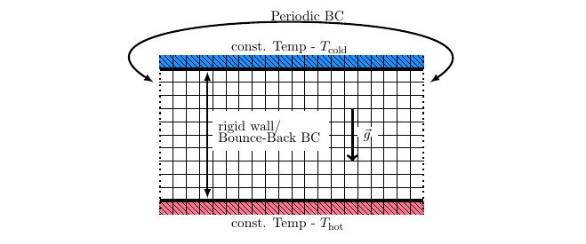
Convection in the Rayleigh-Benard system

Bild
Rayleigh (1916) temperature difference between the upper- and lower-surfaces \[ T(x, y, z=H) = \, T_0 \] \[ T(x, y, z=0) \, = \, T_0 + \Delta T \]
Furthermore \[ \rho = \rho_0 = const. \] except in the buoyancy term, where:
\[ \varrho = \varrho_0 (1 - \alpha(T-T_0)) \mbox{ with } \alpha > 0 \quad . \]
common feature of geophysical flows
No Convection Equilibrium: Diffusion
Bild
Diffusion: Temperature varies linearly with depth:
\[ T_{eq} = T_0 + \left(1 - \frac{z}{H}\right) \Delta T \]
No movement of particles:
\[ u = w= 0 \]
When this solution becomes unstable, convection should develop.
No Convection Equilibrium: Diffusion
Rayleigh-Bénard convection and bifurcation
Experiments:
trailer
Cellules de Bénard (1min),
Rayleigh–Bénard
convection made with mix of cooking oil and small aluminium
particles (5 min),
Was haben
Benard-Zellen mit Kochen zu tun? (3 min, German)
Simulations:
Rayleigh Benard
Thermal Convection with LBM (5 min),
Rayleigh Benard
Thermal Convection 3D Simulation (2 min)
Sketch,
Clouds,
Cartoon
Bifurcations
Bifurcation
youtube (20 min)
Bifurcation Khan
academy (13 min) Reading
Bifurcation theory
Vorticity in the Rayleigh-Benard system
\[ D_t u = - \frac{1}{\rho_0} \partial_x p + \nu \nabla^2 u \label{eqref:einse} \qquad \qquad \qquad \qquad \qquad \qquad (1) \]
\[ D_t w = - \frac{1}{\rho_0} \partial_z p + \nu \nabla^2 w + g (1- \alpha (T-T_0)) \qquad \qquad (2)\]
\[ \partial_x u + \partial_z w = 0 \qquad \qquad \qquad \qquad \qquad \qquad \qquad (3) \]
\[ D_t T = \kappa \nabla^2 T \qquad \qquad \qquad \qquad \qquad \qquad \qquad (4) \]
Introduce vorticity to have (1,2,3) in one equation:
\[ D_t \left( \nabla^2 \Psi\right) = \nu \nabla^4 \Psi - g \alpha \frac{\partial \Theta}{\partial x} \]
Temperature in the Rayleigh-Benard system
\[ T_{eq} = T_0 + \left(1 - \frac{z}{H}\right) \Delta T \]
\[ \mbox{with } \quad T = T_{eq} + \Theta \quad , \quad \mbox{where } \quad \Theta \quad \mbox{is the anomaly} \]
In vorticity equation:
\[ \frac{\partial }{\partial x} g (1- \alpha (T_{eq} + \Theta -T_0)) = - g \alpha \frac{\partial }{\partial x} \Theta \]
Temperature equation:
\[ D_t T = D_t T_{eq} + D_t \Theta = w \cdot \frac{- \Delta T}{H} + D_t \Theta = - \frac{\Delta T}{H} \frac{\partial \Psi}{\partial x} + D_t \Theta \]
\[ D_t \Theta \quad = \frac{\Delta T}{H} \frac{\partial \Psi}{\partial x} + \kappa \nabla^2 \Theta \quad \]
Non-dimensional Rayleigh-Benard system
\[ \frac{1}{T} \frac{1}{L^2} \frac{L^2}{T} D_t \left( \nabla_d^2 \Psi_d\right) = \nu \frac{1}{L^4} \frac{L^2}{T} \nabla_d^4 \Psi_d - g \alpha \frac{ \Delta T}{L} \frac{\partial \Theta_d}{\partial x_d} \]
\[ \frac{\Delta T}{T} D_t \Theta_d \quad = \frac{\Delta T}{H} \frac{L^2}{ T L} \frac{\partial \Psi_d}{\partial x_d} + \kappa \frac{\Delta T}{L^2} \nabla_d^2 \Theta_d \quad \]
This yields (remember \(L=H\))
\[ D_t \left( \nabla_d^2 \Psi_d\right) = \nu \frac{T}{H^2} \nabla_d^4 \Psi_d - g \alpha \frac{T^2 \Delta T}{H} \frac{\partial \Theta_d}{\partial x_d} \]
\[ D_t \Theta_d \quad = \frac{\partial \Psi_d}{\partial x_d} + \kappa \frac{T}{H^2} \nabla_d^2 \Theta_d \quad \]
\[ \mbox{Inserting} \quad T= H^2/\kappa \] \[ \mbox{Rayleigh number} \quad R_a = \frac{g \alpha H^3 \Delta T}{\nu \kappa}\] \[ \mbox{Prandtl number} \quad \sigma = \frac{ \nu}{ \kappa} \]
gives:
\[ D_t \left( \nabla_d^2 \Psi_d\right) = \frac{ \nu}{ \kappa} \nabla_d^4 \Psi_d - g \alpha \frac{H^3 \Delta T}{\kappa^2} \frac{\partial \Theta_d}{\partial x_d} \label{eqref:psieqnn3} \]
\[ D_t \Theta_d \quad = \frac{\partial \Psi_d}{\partial x_d} + \nabla_d^2 \Theta_d \quad . \]
Finally, inserting the non-dimensional parameters
\[ D_t \left( \nabla_d^2 \Psi_d\right) = \sigma \nabla_d^4 \Psi_d - R_a \sigma \frac{\partial \Theta_d}{\partial x_d} \]
\[ D_t \Theta_d \quad = \frac{\partial \Psi_d}{\partial x_d} + \nabla_d^2 \Theta_d \quad \]
Galerkin approximation: Get a low-order model
Bild
\[ \mbox{ Saltzman (1962): Expand } \Psi, \Theta \mbox{ in double Fourier series in x and z: } \]
\[ \Psi (x,z,t) \, = \, \sum_{k=1}^\infty \sum_{l=1}^\infty \Psi_{k,l} (t) \, \, \sin \left(\frac{k \pi a}{H} x \right) \, \times \, \sin \left(\frac{ l \pi}{H} z \right) \] \[ \Theta (x,z,t) \, = \, \sum_{k=1}^\infty \sum_{l=1}^\infty \Theta_{k,l} (t) \cos \left(\frac{k \pi a}{H} x \right) \, \times \, \sin \left( \frac{l \pi}{H} z \right) \]
Approximation: Just 3 Modes X(t), Y(t), Z(t)
\[ \frac{a}{1+a^2} \, \kappa \, \Psi = X \sqrt{2} \sin\left(\frac{\pi a}{H} x \right) \sin\left(\frac{\pi}{H} z \right) \]
\[ \pi \frac{R_a}{R_c} \frac{1}{\Delta T} \, \Theta = Y \sqrt{2} \cos\left(\frac{\pi a}{H} x\right) \sin\left(\frac{\pi}{H} z \right) - Z \sin\left(2 \frac{\pi}{H} z \right) \]
Rayleigh number Ra: Buoyancy & Viscosity
\[ \mbox{Motion develops if } \quad R_a = \frac{g \alpha H^3 \Delta T}{\nu \kappa} \quad \mbox{exceeds } \quad R_c = \pi^4 \frac{(1+a^2)^3}{a^2} \] \[=657.51 \mbox{ occurs when } a^2 = 1/2. \]
\[\mbox{When } R_a < R_c,\mbox{ heat transfer is due to conduction} \]
\[\mbox{When } R_a > R_c, \mbox{ heat transfer is due to convection.} \]
Bild
Lorenz system (also next lecture)
Bifurcation at \[ r = R_a/R_c = 1\]
Geometry constant \[b = 4(1+a^2)^{-1}\]
Famous low-order model:
\[ \dot X = -\sigma X + \sigma Y \]
\[ \dot Y = r X - Y - X Z \]
\[ \dot Z = -b Z + X Y \]
\[\mbox{dimensionless time } \quad t_d = \pi^2 H^{-2} (1+a^2) \kappa t,\]
\[ \mbox{ Prandtl number } \quad \sigma = \nu \kappa^{-1}, \]
Lorenz system r=24
left: 52%
r=24
s=10
b=8/3
dt=0.01
x=0.1
y=0.1
z=0.1
vx<-c(0)
vy<-c(0)
vz<-c(0)
for(i in 1:10000){
x1=x+s*(y-x)*dt
y1=y+(r*x-y-x*z)*dt
z1=z+(x*y-b*z)*dt
vx[i]=x1
vy[i]=y1
vz[i]=z1
x=x1
y=y1
z=z1}
plot(vx,vy,type="l",xlab="x",ylab="y")
plot(vy,vz,type="l",xlab="y",ylab="z")

Lorenz system r=0.9
r=0.9
s=10
b=8/3
dt=0.01
x=1.1
y=0.1
z=11.1
vx<-c(0)
vy<-c(0)
vz<-c(0)
for(i in 1:100){
x1=x+s*(y-x)*dt
y1=y+(r*x-y-x*z)*dt
z1=z+(x*y-b*z)*dt
vx[i]=x1
vy[i]=y1
vz[i]=z1
x=x1
y=y1
z=z1}
plot(vx,type="l",xlab="time",ylab="x")
plot(vy,type="l",xlab="time",ylab="y")

Lorenz system r=3.5
r=3.5
s=10
b=8/3
dt=0.01
x=1.1
y=0.1
z=11.1
vx<-c(0)
vy<-c(0)
vz<-c(0)
for(i in 1:1000){
x1=x+s*(y-x)*dt
y1=y+(r*x-y-x*z)*dt
z1=z+(x*y-b*z)*dt
vx[i]=x1
vy[i]=y1
vz[i]=z1
x=x1
y=y1
z=z1}
plot(vx,type="l",xlab="time",ylab="x")
plot(vy,type="l",xlab="time",ylab="y")

as an outlook: Conveyor Belt

Conveyor
outlook: Thermohaline ocean circulation

Overturning
Modelled meridional overturning streamfunction in Sv 10^6 = m^3 /s in the Atlantic Ocean. Grey areas represent zonally integrated smoothed bathymetry