Dynamics II: lecture 6
Gerrit Lohmann date: May 31, 2021
Organization of
What drives the ocean currents?
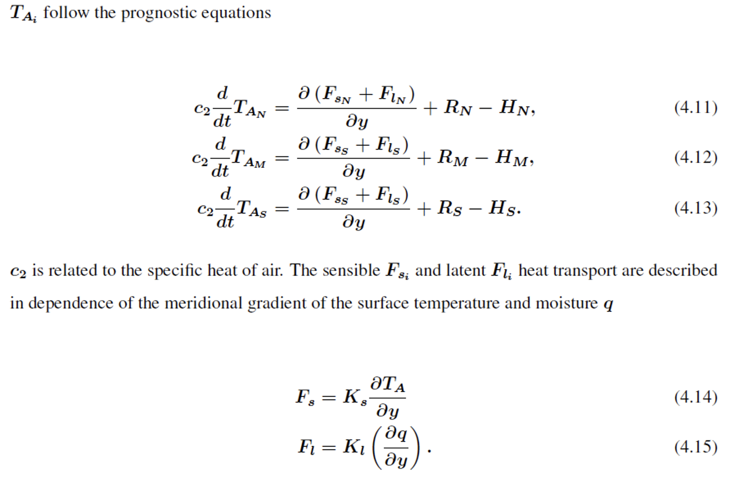
Sverdrup transport
applied globally using the wind stress from Hellerman and Rosenstein (1983). Contour interval is \( 10 \) Sverdrups (Tomczak and Godfrey, 1994).
\[ V = \frac{1}{\rho \beta} \, \left( \frac{\partial \tau_{yz} }{\partial x} \, - \frac{\partial \tau_{xz}}{\partial y}\, \right) = \frac{1}{\rho \beta} \, \, \operatorname{curl} \, \tau \]
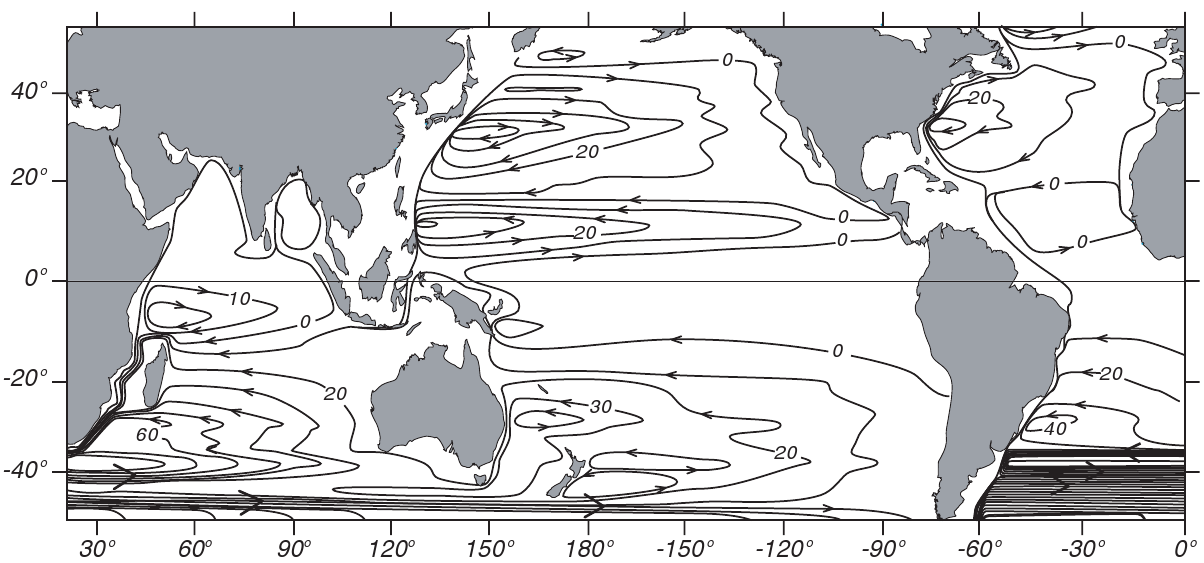
Ekman Pumping: vertical velocity at the bottom
Ekman Pumping & Sverdrup Transport
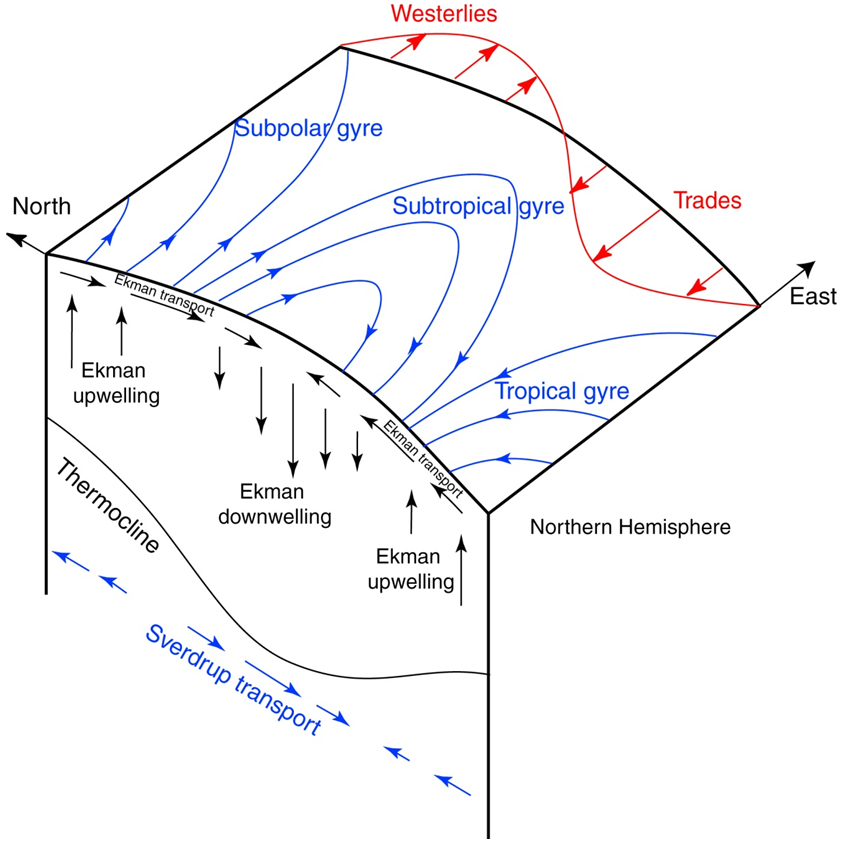
Ocean layers
Steady winds blowing on the sea surface produce a thin, horizontal boundary layer, the Ekman layer. A similar boundary layer exists at the bottom of the atmosphere just above the sea surface, the planetary boundary layer.
North Atlantic Current & Gulfstream
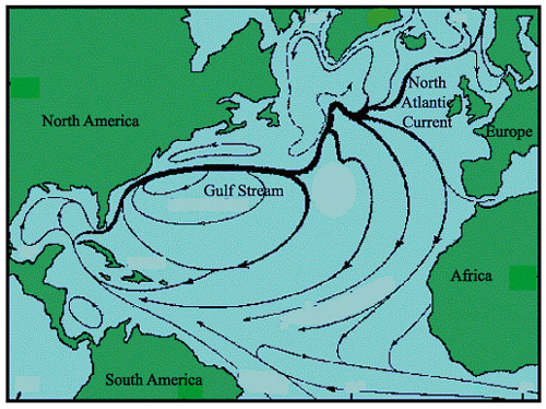
brings warm water northward where it cools.
returns southward as a cold, deep, western-boundary current.
Ocean heat transport
![]()
Conveyor Belt
Ocean: History
Conveyor Belt
Conveyor belt: climate change
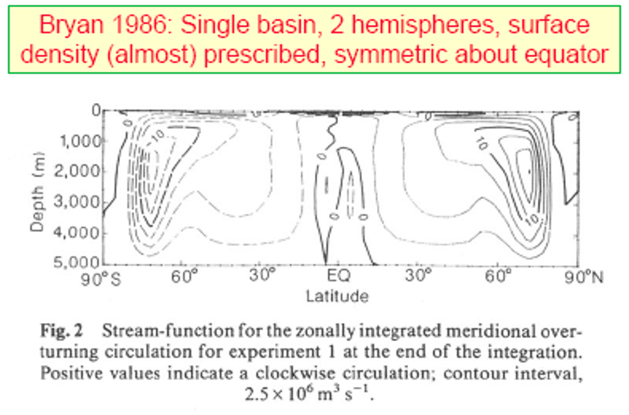
Overturning Circulation (model)
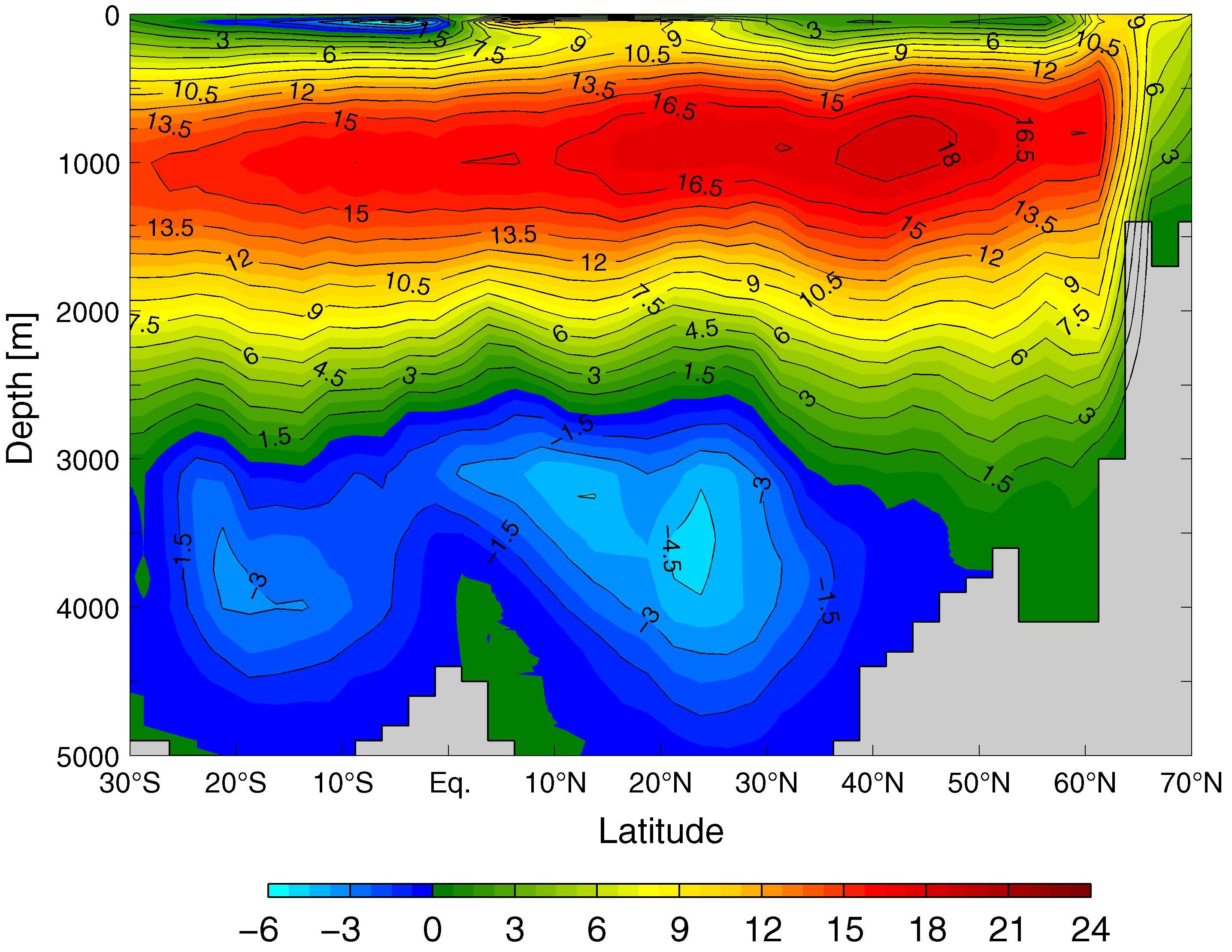 Modelled meridional overturning streamfunction in Sv 106 = m3 /s in the Atlantic Ocean. Grey areas represent zonally integrated smoothed bathymetry
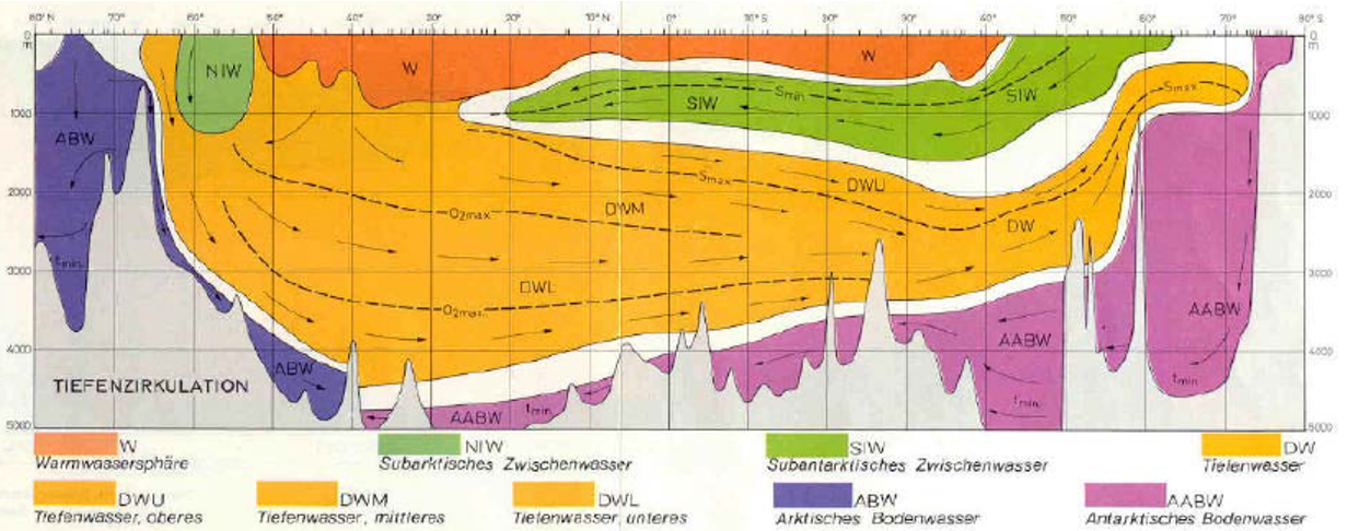
Atlantic water masses
North
Estimates of overturning
Vorticity dynamics of meridional overturning (y,z)
Amplitude of overturning
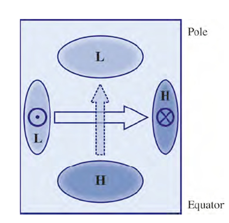
North-south density gradient in an ocean basin
Primary north-south gradient in balance with an eastward geostrophic current: generates a secondary high & low pressure system, northward current
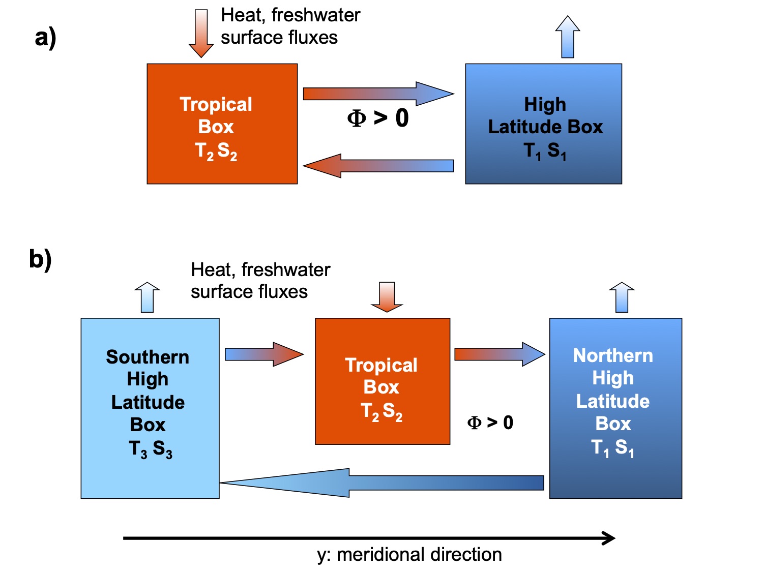
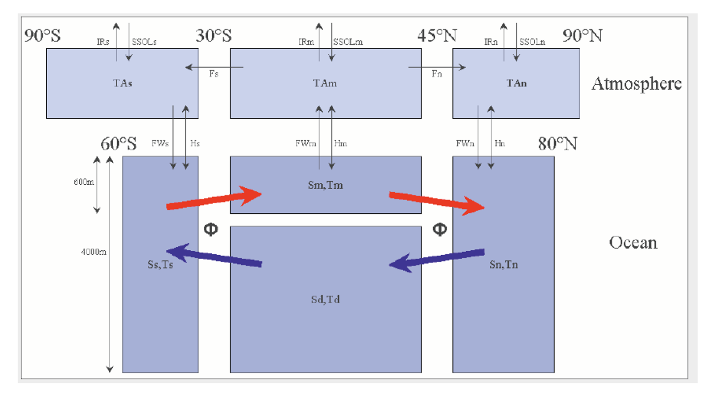
Schematic picture of the hemispheric two box model (a) and of the interhemispheric box model
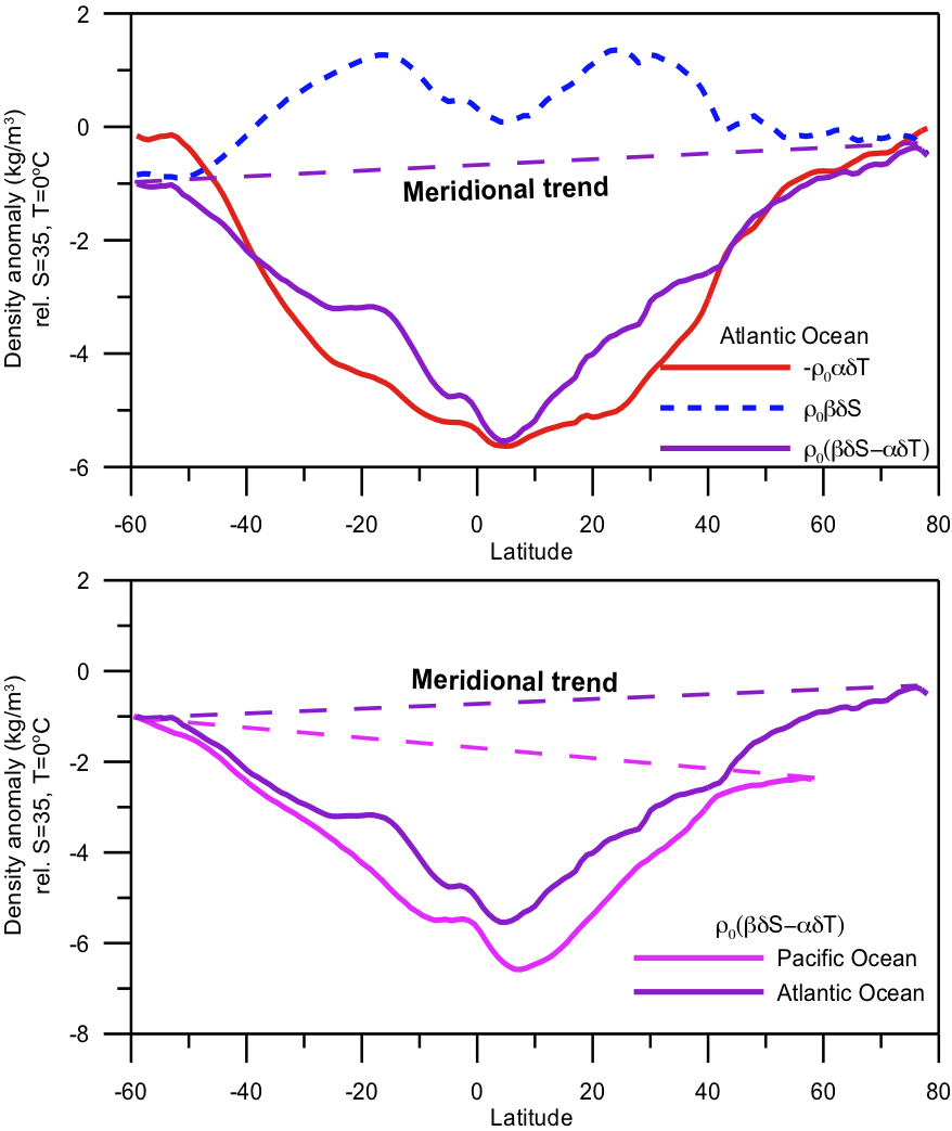
a) The Atlantic surface density is mainly related to temperature differences. b) But the pole-to-pole differences are caused by salinity differences. }
Box model of the thermohaline circulation
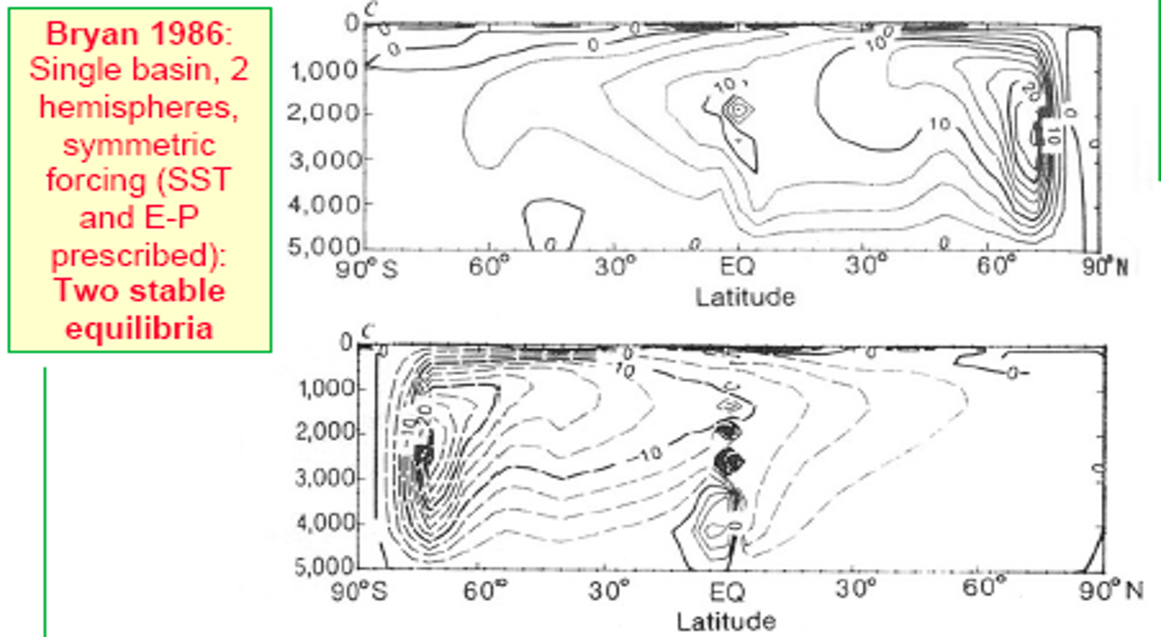
Ocean: multiple equilibria in GCM
Ocean: multiple equilibria in GCM
Ocean response: Hosing the North Atlantic
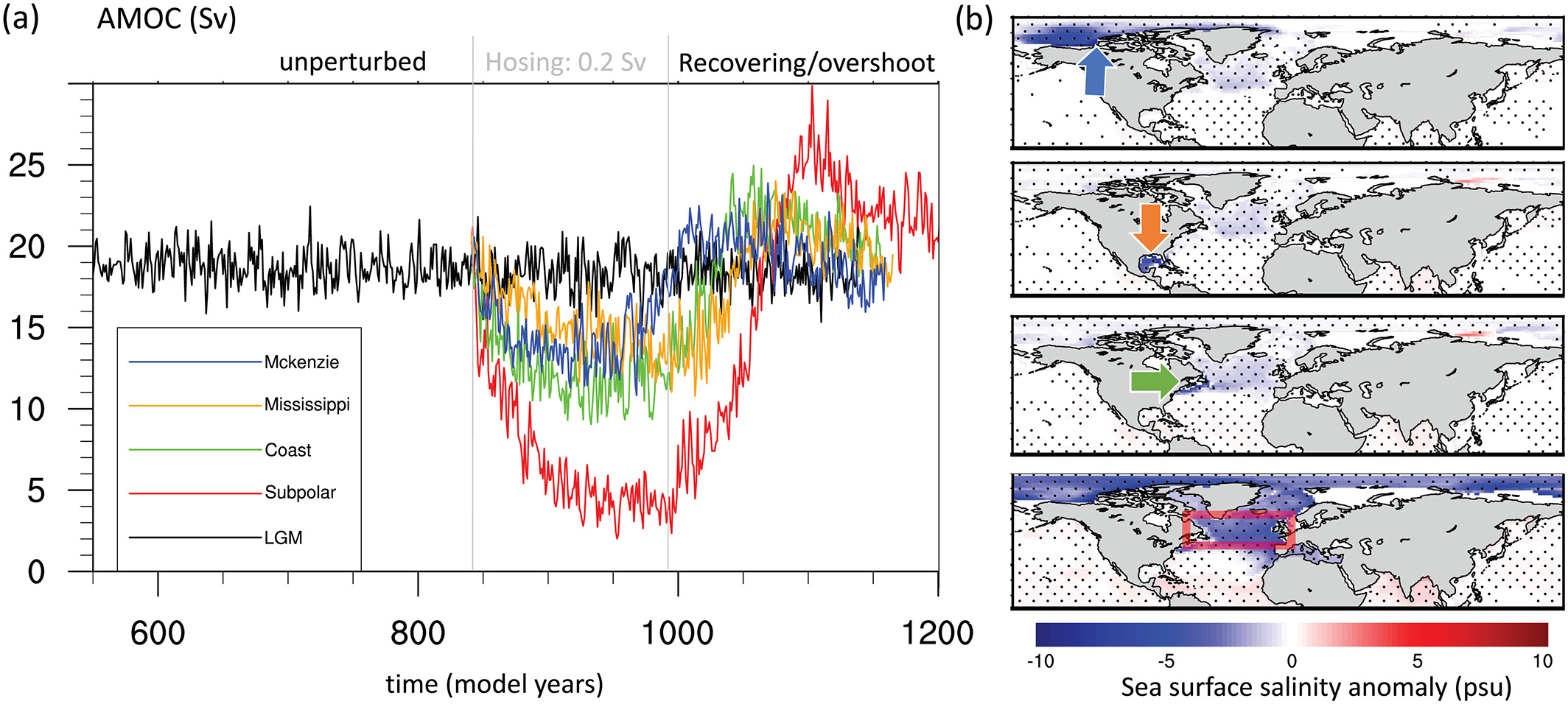
(a) AMOC indices of North Atlantic hosing for different hosing areas. Units are Sv. Black line represents the unperturbed LGM experiment. Hosing is for the period 840–990. (b) Annual mean sea surface salinity anomaly between LGM and the perturbation experiment LGM with 0.2 Sv for the model years 900–950.
-> Multi-scale Ocean GCM
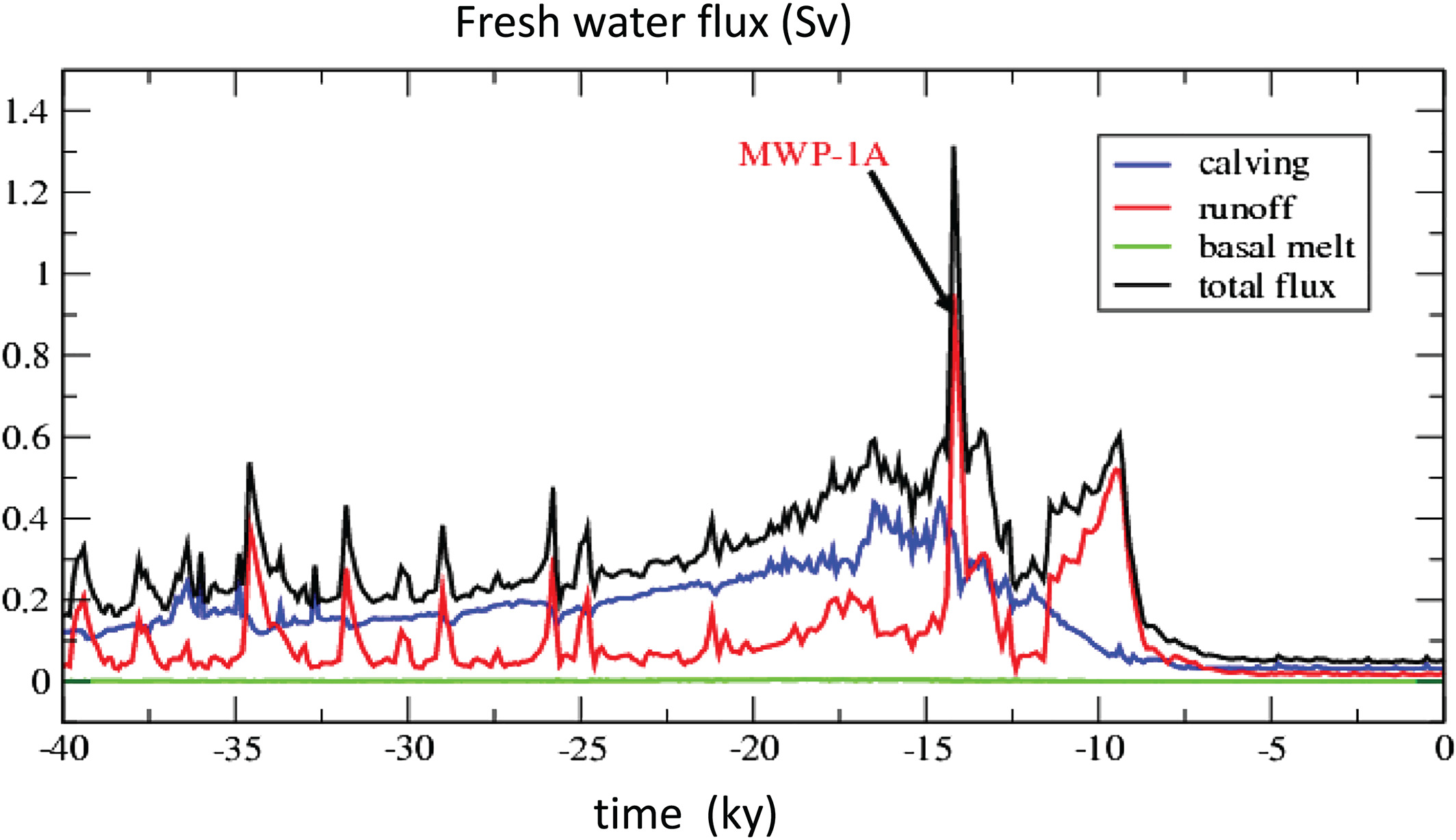
Conveyor belt: climate change
halting or reversing the ocean circulation
interpretation of Greenland ice core records
climate states with different ocean modes
Abrupt climate change, termination of ice sheets, Climate System II
Ocean box model
Ocean: Temperature
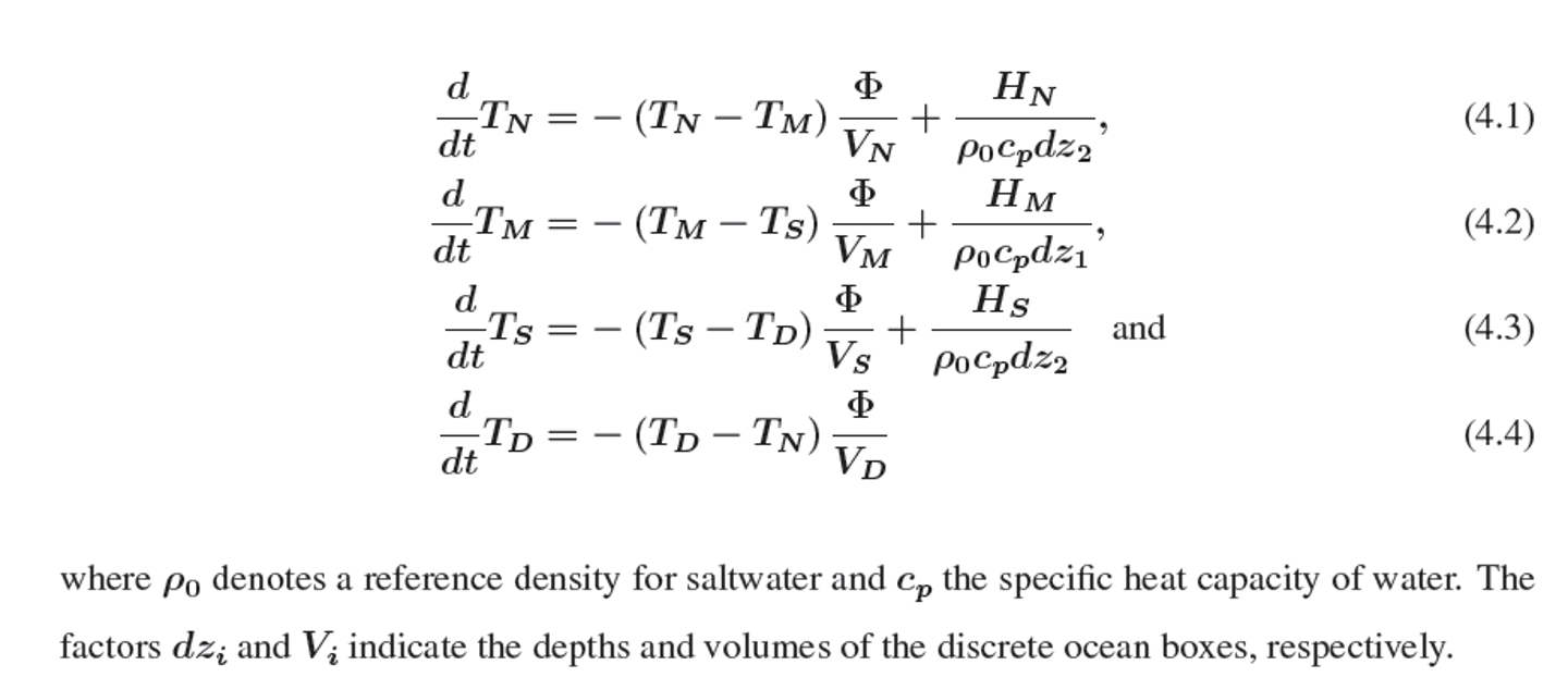
Euler forward for ocean temperature
      Tnln = Tnl + dts * ((Hfnl)/(rcz2)-(Tnl-Tml)*phi/Vnl);

      Tmln = Tml + dts * ((Hfml)/(rcz1)-(Tml-Tsl)*phi/Vml);

      Tsln = Tsl + dts * ((Hfsl)/(rcz2)-(Tsl-Td)*phi/Vsl);

      Tdn = Td + dts * (-(Td-Tnl)*(phi/Vd));
Atmosphere