Dynamics II: lecture 1

Overview of the course: here or local

Content

Fluid dynamics, ocean circulation, wind-driven and thermohaline circulation; atmosphere dynamics, dynamical system theory, non-dimensional parameters, bifurcations and instabilities; Gravity, Rossby, and Kelvin waves; Conceptual models, Analytical and Programming techniques; Time series analysis

Learning outcome

• Advanced dynamics of the ocean and atmosphere, applications in the fields of climate dynamics and fluid mechanics.
• Programming skills (R studio) and usage of the climate data operators.
• Theoretical concepts in physics of climate, temporal and spatial scales of climate dynamics

Lecture: April 12. (Monday), 14:00 Prof. Dr. Gerrit Lohmann

Tutorial: April 12. (Monday), 16:00 Justus Contzen and Lars Ackermann

Time required for Sheet 1: 8 h

Preparation

Chapter The equations of fluid motion (Marchal and Plumb, 2008). (45 min)

Content in the script: Fluid Dynamics, Non-dimensional parameters, Dynamical similarity, Elimination of the pressure term and vorticity

After the lecture: Read the script about Basics of Fluid Dynamics (Chapter 1)

Reading/learning (the sections with a star are voluntary). It might take 60 min.

Content of today's lecture (45 min)

• Fluid Dynamics
• Non-dimensional parameters
• Dynamical similarity
• Elimination of the pressure term and vorticity

Content of today's lecture:

• Fluid Dynamics
• Non-dimensional parameters
• Dynamical similarity
• Elimination of the pressure term and vorticity

Our fluid model describes:

• State variables: Velocity (3D), pressure, temperature, salinity, density, etc.
• Fundamental laws: Conservation of momentum, mass, temperature and salinity
• Equations of state: Relationship of density to temperature, salinity, pressure, etc.

\[ \rho \left( \frac{\partial \mathbf{u}}{\partial t} + \mathbf{u} \cdot \nabla \mathbf{u} \right) = -\nabla p + \nabla \cdot \mathbb{T} + \mathbf{F}, \]

\( \mathbf{u} \) velocity (a vector), \( \rho \) fluid density,

\( p \) pressure, \( \mathbb{T} \) the \( 3\times 3 \) (deviatoric) stress tensor,

\( \mathbf{F} \) represents body forces (per unit volume) acting on the fluid.

\[ \rho \left( \frac{\partial \mathbf{u}}{\partial t} + \mathbf{u} \cdot \nabla \mathbf{u} \right) = -\nabla p + \nabla \cdot \mathbb{T} + \mathbf{F}, \]

\( \mathbf{u} \) velocity (a vector), \( \rho \) fluid density,

\( p \) pressure, \( \mathbb{T} \) the \( 3\times 3 \) (deviatoric) stress tensor,

\( \mathbf{F} \) represents body forces (per unit volume) acting on the fluid.

This equation is often written using the substantive derivative (a statement of Newton's second law):

\[ \rho \frac{D \mathbf{u}}{D t} = -\nabla p + \nabla \cdot\mathbb{T} + \mathbf{F} \label{newtonzwei} \]

\[ \overbrace{\rho \Big( \underbrace{\frac{\partial \mathbf{u}}{\partial t}}_{ \begin{smallmatrix} \text{Unsteady}\\ \text{acceleration} \end{smallmatrix}} + \underbrace{\mathbf{u} \cdot \nabla \mathbf{u}}_{ \begin{smallmatrix} \text{Advective} \\ \text{acceleration} \end{smallmatrix}}\Big)}^{\text{Inertia (per volume)}} = \overbrace{\underbrace{-\nabla p}_{ \begin{smallmatrix} \text{Pressure} \\ \text{gradient} \end{smallmatrix}} + \underbrace{\nabla \cdot\mathbb{T}}_{\text{Viscosity}}}^{\text{Divergence of stress}} + \underbrace{\mathbf{F}}_{ \begin{smallmatrix} \text{Other} \\ \text{body} \\ \text{forces} \end{smallmatrix}} \]

\[ \overbrace{\rho \Big( \underbrace{\frac{\partial \mathbf{u}}{\partial t}}_{ \begin{smallmatrix} \text{Unsteady}\\ \text{acceleration} \end{smallmatrix}} + \underbrace{\mathbf{u} \cdot \nabla \mathbf{u}}_{ \begin{smallmatrix} \text{Advective} \\ \text{acceleration} \end{smallmatrix}}\Big)}^{\text{Inertia (per volume)}} = \overbrace{\underbrace{-\nabla p}_{ \begin{smallmatrix} \text{Pressure} \\ \text{gradient} \end{smallmatrix}} + \underbrace{\nabla \cdot\mathbb{T}}_{\text{Viscosity}}}^{\text{Divergence of stress}} + \underbrace{\mathbf{F}}_{ \begin{smallmatrix} \text{Other} \\ \text{body} \\ \text{forces} \end{smallmatrix}} \]

A very significant feature of the Navier-Stokes equations is the presence of advective acceleration:

\[ \mathbf{u} \cdot \nabla \mathbf{u} \]

(Script: A general framework as transport phenomenon.)

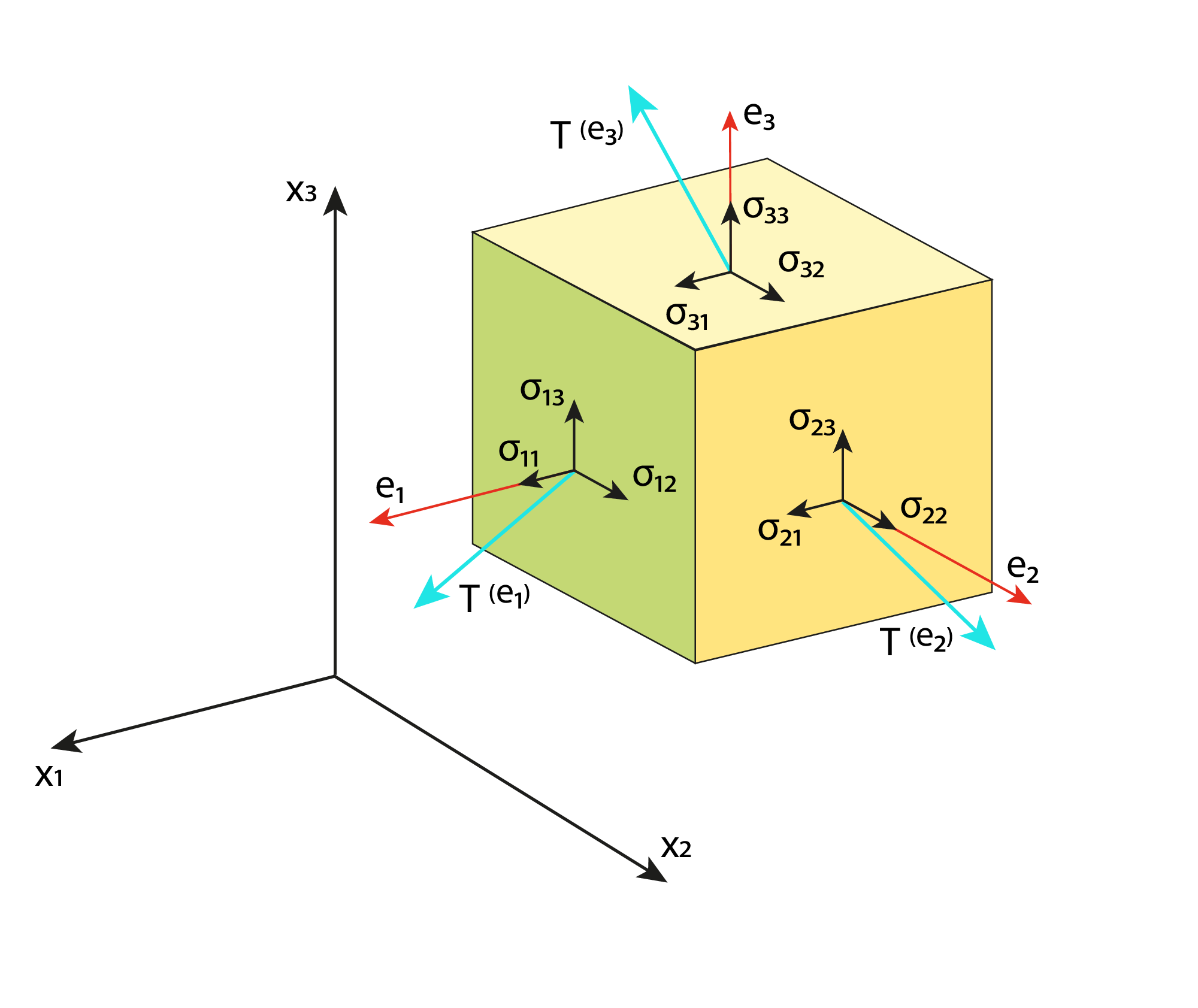Components of stress in three dimensions.

\( \nabla p \) pressure gradient: isotropic part

\( \nabla \cdot\mathbb{T} \) anisotropic part describing viscous forces.

Model is needed relating the stresses to the fluid motion

Cauchy stress tensor: \[ \mathbb{T} = \left({\begin{matrix} \mathbf{T}^{(\mathbf{e}_1)} \\ \mathbf{T}^{(\mathbf{e}_2)} \\ \mathbf{T}^{(\mathbf{e}_3)} \\ \end{matrix}}\right) = \left({\begin{matrix} \sigma _{11} & \sigma _{12} & \sigma _{13} \\ \sigma _{21} & \sigma _{22} & \sigma _{23} \\ \sigma _{31} & \sigma _{32} & \sigma _{33} \\ \end{matrix}}\right) \equiv \left({\begin{matrix} \sigma _x & \tau _{xy} & \tau _{xz} \\ \tau _{yx} & \sigma _y & \tau _{yz} \\ \tau _{zx} & \tau _{zy} & \sigma _z \\ \end{matrix}}\right) \]

\( \tau \) are the shear stresses, and \( p=-{\frac{1}{3}}(\sigma_{x}+\sigma_{y}+\sigma_{z}) \)

From the Newton's third law (actio est reactio), symmetry \[ \mathbb{T} = \mathbb{T}^T \]

Components of stress in three dimensions.

Regardless of the flow assumptions, a statement of the conservation of mass is generally necessary. This is achieved through the mass continuity equation, given in its most general form as: \[ \frac{\partial \rho}{\partial t} + \nabla \cdot (\rho \mathbf{u}) = 0 \]

or, using the substantive derivative:

\[ \frac{D\rho}{Dt} + \rho (\nabla \cdot \mathbf{u}) = 0. \]

The temperature at a point 50 km north of a station is \( 3^oC \) cooler than at the station.

If the wind is blowing from the northeast at 20m/s

and the air is being heated by radiation at a rate of \( 1^oC/h \).

What is the local temperature change at the station?

The total change of temperature is given by

\[ \frac{d T}{dt} = \frac{\partial T}{\partial t} + {\bf u} \cdot \nabla T = \dot{q} \quad \Leftrightarrow \quad \frac{\partial T}{\partial t} = - {\bf u} \cdot \nabla T + \dot{q} \]

Here we use the velocity (from northeast)

\[ {\bf u} = - 20 \frac{m}{s} \cdot \frac{1}{\sqrt{2}} (1, 1, 0) , \quad \nabla T = \frac{{3}{^\circ C}}{{50}{km}} (0, -1, 0), \quad \dot{q} = 1 \frac{^\circ C}{h} \]

Then we calculate the temperature change at the station

\[ \frac{\partial T}{\partial t} = 20 \frac{m}{s} \, \frac{1}{\sqrt{2}} (1, 1, 0) \cdot (0, -1, 0) \frac{{3}{^\circ C}}{{50}{km}} + 1 \frac{^\circ C}{h} \approx {-2.1} \frac{^\circ C}{h} \]

\( \nabla \cdot \mathbb{T} \) becomes \( \mu \nabla^2 \mathbf{u} \) with \( \mu \) dynamic viscosity.

\[ \rho \left(\frac{\partial \mathbf{u}}{\partial t} + \mathbf{u} \cdot \nabla \mathbf{u}\right) = -\nabla p + \mu \nabla^2 \mathbf{u} + \mathbf{F}. \label{reyn0} \]

The vector field \( \mathbf{F} \) represents “other” (body force) forces. Typically gravity, but may include other fields (such as electromagnetic).

Often, these forces may be represented as the gradient of some scalar quantity. E.g.: Gravity in the z direction is the gradient of \( - \rho gz \)

Since pressure shows up only as a gradient, this implies that solving a problem without any such body force: include the body force by modifying pressure

\[ \overbrace{\rho \Big( \underbrace{\frac{\partial \mathbf{u}}{\partial t}}_{ \begin{smallmatrix} \text{Unsteady}\\ \text{acceleration} \end{smallmatrix}} + \underbrace{\mathbf{u} \cdot \nabla \mathbf{u}}_{ \begin{smallmatrix} \text{Advective} \\ \text{acceleration} \end{smallmatrix}}\Big)}^{\text{Inertia (per volume)}} = \overbrace{\underbrace{-\nabla p}_{ \begin{smallmatrix} \text{Pressure} \\ \text{gradient} \end{smallmatrix}} + \underbrace{\mu \nabla^2 \mathbf{u}}_{\text{Viscosity}}}^{\text{Divergence of stress}} + \underbrace{\mathbf{F}}_{ \begin{smallmatrix} \text{Other} \\ \text{body} \\ \text{forces} \end{smallmatrix}} \]

If temperature effects are also neglected, the only “other” equation: mass continuity equation. Under the incompressible assumption, density is a constant and it follows that the equation will simplify to:

\[ \nabla \cdot \mathbf{u} = 0 \qquad . \label{consmass} \]

This becomes a statement of the conservation of volume !

2D: assume \( w = 0 \) and no dependence of anything on z

\[ \rho \left(\frac{\partial u}{\partial t} + u \frac{\partial u}{\partial x} + v \frac{\partial u}{\partial y}\right) = -\frac{\partial p}{\partial x} + \mu \left(\frac{\partial^2 u}{\partial x^2} + \frac{\partial^2 u}{\partial y^2}\right) \] \[ \rho \left(\frac{\partial v}{\partial t} + u \frac{\partial v}{\partial x} + v \frac{\partial v}{\partial y}\right) = -\frac{\partial p}{\partial y} + \mu \left(\frac{\partial^2 v}{\partial x^2} + \frac{\partial^2 v}{\partial y^2}\right) \]

Procedure

• Differentiating the first with respect to y: \( \quad \partial_y \)

• the second with respect to x: \( \quad \partial_x \)

• and subtracting the resulting equations will eliminate pressure and any potential force.

Defining the stream function through \[ u = \frac{\partial \psi}{\partial y} \quad ; \quad v = -\frac{\partial \psi}{\partial x} \]

results in mass continuity being unconditionally satisfied:

\[ \frac{\partial}{\partial t}\left(\nabla^2 \psi\right) + \frac{\partial \psi}{\partial y} \frac{\partial}{\partial x}\left(\nabla^2 \psi\right) - \frac{\partial \psi}{\partial x} \frac{\partial}{\partial y}\left(\nabla^2 \psi\right) = \nu \nabla^4 \psi \]

or using the total derivative

\[ D_t \left(\nabla^2 \psi\right) = \nu \nabla^4 \psi \]

\( \nu \) the kinematic viscosity \( \nu=\frac{\mu}{\rho}. \)

This single equation describes 2D fluid flow !

kinematic viscosity as parameter!

incompressible flow, temperature effects are negligible and external forces are neglected.

conservation of mass \[ \nabla \cdot \mathbf{u} = 0 \] conservation of momentum \[ \partial_t \mathbf{u} + ( \mathbf{u} \cdot \nabla) \mathbf{u} = - \frac{1}{\rho_0} \nabla p + \nu \nabla^2 \mathbf{u} \]

The equations can be made dimensionless by a length-scale L, determined by the geometry of the flow, and by a characteristic velocity U.

For analytical solutions, numerical results, and experimental measurements, it is useful to report the results in a dimensionless system (concept of dynamic similarity).

Goal: replace physical parameters with dimensionless numbers, which completely determine the dynamical behavior

Representative values for velocity (U), time (T), distances (L). Using these values, the values in the dimensionless-system (written with subscript d) can be defined: \[ u =U \cdot u_d \] \[ t = T \cdot t_d \] \[ x = L \cdot x_d \] with \( U = L/T \).

From these scalings, we can also derive

\[ \partial_t = \frac{\partial}{\partial t } = \frac{1}{T} \cdot \frac{\partial}{\partial t_d } \] \[ \partial_x = \frac{\partial}{\partial x} = \frac{1}{L} \cdot \frac{\partial}{\partial x_d } \]

Note furthermore the units of \( [\rho_0] = kg/m^3, [p] = kg/(m s^2), [p]/[\rho_0]= {m^2}/{s^2} \)

Therefore the pressure gradient term has the scaling \( U^2/L \).

\[ \nabla_d \cdot \mathbf{u_d} = 0 \] and conservation of momentum \[ \frac{\partial}{\partial t_d } \mathbf{u_d} + ( \mathbf{u_d} \cdot \nabla_d) \mathbf{u_d} = - \nabla_d p_d + \frac{1}{Re} \nabla_d^2 \mathbf{u_d} \] The dimensionless parameter \[ Re=UL/ \nu \]

is the Reynolds number and the only parameter left!

For large Reynolds numbers, the flow is turbulent. \( Re \sim (10^4-10^8) \). Flow develops steep gradients locally.

In the literature: “equations have been made dimensionless”, means that our procedure is applied and the subscripts d are dropped.

These numbers can be interpreted as follows:

• Re: (stationary inertial forces)/(viscous forces)
• Sr: (non-stationary inertial forces)/(stationary inertial forces)
• Fr: (stationary inertial forces)/(gravity)
• Fo: (heat conductance)/(non-stationary change in enthalpy)
• Pe: (convective heat transport)/(heat conductance)
• Ec: (viscous dissipation)/(convective heat transport)
• Ma: (velocity)/(speed of sound): objects moving faster than 0.8 produce shockwaves
• Pr and Nu are related to specific materials.

• Fluid Dynamics, Non-dimensional parameters
• Dynamical similarity
• Elimination of the pressure term and vorticity

After the lecture: Read the script about Basics of Fluid Dynamics (Chapter 1)

Reading/learning might take 45 min.

Watch the video Introduction to Atmospheric Dynamics (47 min)

based on Chapter 1 from Holton and Hakim (2013)

After the video: Read Introduction to Atmospheric Dynamics (Chapter 1)

Reading/learning might take 60 min.

Workload /credit points: 3 CP, 90 h

• lecture: 24 h (2h x 12 weeks)
• repeating the lectures/learning/reading: 24 h (2h x 12 weeks)
• example classes: 11 h (1h x 11 weeks)
• example classes homework: 20 h (2h x 10 weeks)
• additional preparation for exam: 11 h

Course achievements:

50% of the points of the exercise sheets are required. Furthermore, we require active participation with at least one time showing a solution in the chat room. Working in study groups is encouraged, but each student is responsible for his/her own solution. If the solution is typewritten (e.g. with LaTex, Rmarkdown, or word), we allow up to 3 persons to be listed on a solution sheet.

Examination achievements:

The exam is based on the exercises and the general content of the lecture. The procedure follows the rules of pep.